Free Statistics
of Irreproducible Research!
Description of Statistical Computation | |||||||||||||||||||||||||||||||||||||||||||||||||||||||||||||||||||||||||||||||||||||||||||||||||||||||||||||||||||||||||||||||||||||||||||||||||||||||||||||||||||||||||||||||||||||||||||||||||||||||||||||||||||||||||||||||||||||||||||||||||||||||||||||||||||||||||||||||||||||||||||||||||||||||||||||||||||||||||||||||||||||||||||||||||||||||||||||||||||||||||||||||||||||||||||||||||||||||||||||||||||||||||||||||||||||||||||||||||||||||||||||||||||||||||||||||||||||||||||||||||||||||||||||||||||||||||||||||||||||||||||||||||||||||||||||
|---|---|---|---|---|---|---|---|---|---|---|---|---|---|---|---|---|---|---|---|---|---|---|---|---|---|---|---|---|---|---|---|---|---|---|---|---|---|---|---|---|---|---|---|---|---|---|---|---|---|---|---|---|---|---|---|---|---|---|---|---|---|---|---|---|---|---|---|---|---|---|---|---|---|---|---|---|---|---|---|---|---|---|---|---|---|---|---|---|---|---|---|---|---|---|---|---|---|---|---|---|---|---|---|---|---|---|---|---|---|---|---|---|---|---|---|---|---|---|---|---|---|---|---|---|---|---|---|---|---|---|---|---|---|---|---|---|---|---|---|---|---|---|---|---|---|---|---|---|---|---|---|---|---|---|---|---|---|---|---|---|---|---|---|---|---|---|---|---|---|---|---|---|---|---|---|---|---|---|---|---|---|---|---|---|---|---|---|---|---|---|---|---|---|---|---|---|---|---|---|---|---|---|---|---|---|---|---|---|---|---|---|---|---|---|---|---|---|---|---|---|---|---|---|---|---|---|---|---|---|---|---|---|---|---|---|---|---|---|---|---|---|---|---|---|---|---|---|---|---|---|---|---|---|---|---|---|---|---|---|---|---|---|---|---|---|---|---|---|---|---|---|---|---|---|---|---|---|---|---|---|---|---|---|---|---|---|---|---|---|---|---|---|---|---|---|---|---|---|---|---|---|---|---|---|---|---|---|---|---|---|---|---|---|---|---|---|---|---|---|---|---|---|---|---|---|---|---|---|---|---|---|---|---|---|---|---|---|---|---|---|---|---|---|---|---|---|---|---|---|---|---|---|---|---|---|---|---|---|---|---|---|---|---|---|---|---|---|---|---|---|---|---|---|---|---|---|---|---|---|---|---|---|---|---|---|---|---|---|---|---|---|---|---|---|---|---|---|---|---|---|---|---|---|---|---|---|---|---|---|---|---|---|---|---|---|---|---|---|---|---|---|---|---|---|---|---|---|---|---|---|---|---|---|---|---|---|---|---|---|---|---|---|---|---|---|---|---|---|---|---|---|---|---|---|---|---|---|---|---|---|---|---|---|---|---|---|---|---|---|---|---|---|---|---|---|---|---|---|---|---|---|---|---|---|---|---|---|---|---|---|---|---|---|---|---|---|---|---|---|---|---|---|---|---|---|---|---|---|---|---|---|---|---|---|---|---|---|---|---|---|---|---|---|---|---|---|---|---|---|---|---|---|---|---|---|---|---|---|---|---|---|
| Author's title | |||||||||||||||||||||||||||||||||||||||||||||||||||||||||||||||||||||||||||||||||||||||||||||||||||||||||||||||||||||||||||||||||||||||||||||||||||||||||||||||||||||||||||||||||||||||||||||||||||||||||||||||||||||||||||||||||||||||||||||||||||||||||||||||||||||||||||||||||||||||||||||||||||||||||||||||||||||||||||||||||||||||||||||||||||||||||||||||||||||||||||||||||||||||||||||||||||||||||||||||||||||||||||||||||||||||||||||||||||||||||||||||||||||||||||||||||||||||||||||||||||||||||||||||||||||||||||||||||||||||||||||||||||||||||||||
| Author | *Unverified author* | ||||||||||||||||||||||||||||||||||||||||||||||||||||||||||||||||||||||||||||||||||||||||||||||||||||||||||||||||||||||||||||||||||||||||||||||||||||||||||||||||||||||||||||||||||||||||||||||||||||||||||||||||||||||||||||||||||||||||||||||||||||||||||||||||||||||||||||||||||||||||||||||||||||||||||||||||||||||||||||||||||||||||||||||||||||||||||||||||||||||||||||||||||||||||||||||||||||||||||||||||||||||||||||||||||||||||||||||||||||||||||||||||||||||||||||||||||||||||||||||||||||||||||||||||||||||||||||||||||||||||||||||||||||||||||||
| R Software Module | rwasp_Mixed Model ANOVA.wasp | ||||||||||||||||||||||||||||||||||||||||||||||||||||||||||||||||||||||||||||||||||||||||||||||||||||||||||||||||||||||||||||||||||||||||||||||||||||||||||||||||||||||||||||||||||||||||||||||||||||||||||||||||||||||||||||||||||||||||||||||||||||||||||||||||||||||||||||||||||||||||||||||||||||||||||||||||||||||||||||||||||||||||||||||||||||||||||||||||||||||||||||||||||||||||||||||||||||||||||||||||||||||||||||||||||||||||||||||||||||||||||||||||||||||||||||||||||||||||||||||||||||||||||||||||||||||||||||||||||||||||||||||||||||||||||||
| Title produced by software | Mixed Within-Between Two-Way ANOVA | ||||||||||||||||||||||||||||||||||||||||||||||||||||||||||||||||||||||||||||||||||||||||||||||||||||||||||||||||||||||||||||||||||||||||||||||||||||||||||||||||||||||||||||||||||||||||||||||||||||||||||||||||||||||||||||||||||||||||||||||||||||||||||||||||||||||||||||||||||||||||||||||||||||||||||||||||||||||||||||||||||||||||||||||||||||||||||||||||||||||||||||||||||||||||||||||||||||||||||||||||||||||||||||||||||||||||||||||||||||||||||||||||||||||||||||||||||||||||||||||||||||||||||||||||||||||||||||||||||||||||||||||||||||||||||||
| Date of computation | Thu, 02 Feb 2012 07:28:45 -0500 | ||||||||||||||||||||||||||||||||||||||||||||||||||||||||||||||||||||||||||||||||||||||||||||||||||||||||||||||||||||||||||||||||||||||||||||||||||||||||||||||||||||||||||||||||||||||||||||||||||||||||||||||||||||||||||||||||||||||||||||||||||||||||||||||||||||||||||||||||||||||||||||||||||||||||||||||||||||||||||||||||||||||||||||||||||||||||||||||||||||||||||||||||||||||||||||||||||||||||||||||||||||||||||||||||||||||||||||||||||||||||||||||||||||||||||||||||||||||||||||||||||||||||||||||||||||||||||||||||||||||||||||||||||||||||||||
| Cite this page as follows | Statistical Computations at FreeStatistics.org, Office for Research Development and Education, URL https://freestatistics.org/blog/index.php?v=date/2012/Feb/02/t1328185738ysu91kk0nlvzdhy.htm/, Retrieved Sun, 31 May 2026 18:27:35 +0000 | ||||||||||||||||||||||||||||||||||||||||||||||||||||||||||||||||||||||||||||||||||||||||||||||||||||||||||||||||||||||||||||||||||||||||||||||||||||||||||||||||||||||||||||||||||||||||||||||||||||||||||||||||||||||||||||||||||||||||||||||||||||||||||||||||||||||||||||||||||||||||||||||||||||||||||||||||||||||||||||||||||||||||||||||||||||||||||||||||||||||||||||||||||||||||||||||||||||||||||||||||||||||||||||||||||||||||||||||||||||||||||||||||||||||||||||||||||||||||||||||||||||||||||||||||||||||||||||||||||||||||||||||||||||||||||||
| Statistical Computations at FreeStatistics.org, Office for Research Development and Education, URL https://freestatistics.org/blog/index.php?pk=161628, Retrieved Sun, 31 May 2026 18:27:35 +0000 | |||||||||||||||||||||||||||||||||||||||||||||||||||||||||||||||||||||||||||||||||||||||||||||||||||||||||||||||||||||||||||||||||||||||||||||||||||||||||||||||||||||||||||||||||||||||||||||||||||||||||||||||||||||||||||||||||||||||||||||||||||||||||||||||||||||||||||||||||||||||||||||||||||||||||||||||||||||||||||||||||||||||||||||||||||||||||||||||||||||||||||||||||||||||||||||||||||||||||||||||||||||||||||||||||||||||||||||||||||||||||||||||||||||||||||||||||||||||||||||||||||||||||||||||||||||||||||||||||||||||||||||||||||||||||||||
| QR Codes: | |||||||||||||||||||||||||||||||||||||||||||||||||||||||||||||||||||||||||||||||||||||||||||||||||||||||||||||||||||||||||||||||||||||||||||||||||||||||||||||||||||||||||||||||||||||||||||||||||||||||||||||||||||||||||||||||||||||||||||||||||||||||||||||||||||||||||||||||||||||||||||||||||||||||||||||||||||||||||||||||||||||||||||||||||||||||||||||||||||||||||||||||||||||||||||||||||||||||||||||||||||||||||||||||||||||||||||||||||||||||||||||||||||||||||||||||||||||||||||||||||||||||||||||||||||||||||||||||||||||||||||||||||||||||||||||
|
| |||||||||||||||||||||||||||||||||||||||||||||||||||||||||||||||||||||||||||||||||||||||||||||||||||||||||||||||||||||||||||||||||||||||||||||||||||||||||||||||||||||||||||||||||||||||||||||||||||||||||||||||||||||||||||||||||||||||||||||||||||||||||||||||||||||||||||||||||||||||||||||||||||||||||||||||||||||||||||||||||||||||||||||||||||||||||||||||||||||||||||||||||||||||||||||||||||||||||||||||||||||||||||||||||||||||||||||||||||||||||||||||||||||||||||||||||||||||||||||||||||||||||||||||||||||||||||||||||||||||||||||||||||||||||||||
| Original text written by user: | |||||||||||||||||||||||||||||||||||||||||||||||||||||||||||||||||||||||||||||||||||||||||||||||||||||||||||||||||||||||||||||||||||||||||||||||||||||||||||||||||||||||||||||||||||||||||||||||||||||||||||||||||||||||||||||||||||||||||||||||||||||||||||||||||||||||||||||||||||||||||||||||||||||||||||||||||||||||||||||||||||||||||||||||||||||||||||||||||||||||||||||||||||||||||||||||||||||||||||||||||||||||||||||||||||||||||||||||||||||||||||||||||||||||||||||||||||||||||||||||||||||||||||||||||||||||||||||||||||||||||||||||||||||||||||||
| IsPrivate? | No (this computation is public) | ||||||||||||||||||||||||||||||||||||||||||||||||||||||||||||||||||||||||||||||||||||||||||||||||||||||||||||||||||||||||||||||||||||||||||||||||||||||||||||||||||||||||||||||||||||||||||||||||||||||||||||||||||||||||||||||||||||||||||||||||||||||||||||||||||||||||||||||||||||||||||||||||||||||||||||||||||||||||||||||||||||||||||||||||||||||||||||||||||||||||||||||||||||||||||||||||||||||||||||||||||||||||||||||||||||||||||||||||||||||||||||||||||||||||||||||||||||||||||||||||||||||||||||||||||||||||||||||||||||||||||||||||||||||||||||
| User-defined keywords | |||||||||||||||||||||||||||||||||||||||||||||||||||||||||||||||||||||||||||||||||||||||||||||||||||||||||||||||||||||||||||||||||||||||||||||||||||||||||||||||||||||||||||||||||||||||||||||||||||||||||||||||||||||||||||||||||||||||||||||||||||||||||||||||||||||||||||||||||||||||||||||||||||||||||||||||||||||||||||||||||||||||||||||||||||||||||||||||||||||||||||||||||||||||||||||||||||||||||||||||||||||||||||||||||||||||||||||||||||||||||||||||||||||||||||||||||||||||||||||||||||||||||||||||||||||||||||||||||||||||||||||||||||||||||||||
| Estimated Impact | 486 | ||||||||||||||||||||||||||||||||||||||||||||||||||||||||||||||||||||||||||||||||||||||||||||||||||||||||||||||||||||||||||||||||||||||||||||||||||||||||||||||||||||||||||||||||||||||||||||||||||||||||||||||||||||||||||||||||||||||||||||||||||||||||||||||||||||||||||||||||||||||||||||||||||||||||||||||||||||||||||||||||||||||||||||||||||||||||||||||||||||||||||||||||||||||||||||||||||||||||||||||||||||||||||||||||||||||||||||||||||||||||||||||||||||||||||||||||||||||||||||||||||||||||||||||||||||||||||||||||||||||||||||||||||||||||||||
Tree of Dependent Computations | |||||||||||||||||||||||||||||||||||||||||||||||||||||||||||||||||||||||||||||||||||||||||||||||||||||||||||||||||||||||||||||||||||||||||||||||||||||||||||||||||||||||||||||||||||||||||||||||||||||||||||||||||||||||||||||||||||||||||||||||||||||||||||||||||||||||||||||||||||||||||||||||||||||||||||||||||||||||||||||||||||||||||||||||||||||||||||||||||||||||||||||||||||||||||||||||||||||||||||||||||||||||||||||||||||||||||||||||||||||||||||||||||||||||||||||||||||||||||||||||||||||||||||||||||||||||||||||||||||||||||||||||||||||||||||||
| Family? (F = Feedback message, R = changed R code, M = changed R Module, P = changed Parameters, D = changed Data) | |||||||||||||||||||||||||||||||||||||||||||||||||||||||||||||||||||||||||||||||||||||||||||||||||||||||||||||||||||||||||||||||||||||||||||||||||||||||||||||||||||||||||||||||||||||||||||||||||||||||||||||||||||||||||||||||||||||||||||||||||||||||||||||||||||||||||||||||||||||||||||||||||||||||||||||||||||||||||||||||||||||||||||||||||||||||||||||||||||||||||||||||||||||||||||||||||||||||||||||||||||||||||||||||||||||||||||||||||||||||||||||||||||||||||||||||||||||||||||||||||||||||||||||||||||||||||||||||||||||||||||||||||||||||||||||
| - [Mixed Within-Between Two-Way ANOVA] [Mixed Within-Betw...] [2012-01-30 17:15:20] [98fd0e87c3eb04e0cc2efde01dbafab6] - R [Mixed Within-Between Two-Way ANOVA] [] [2012-02-02 12:28:45] [d41d8cd98f00b204e9800998ecf8427e] [Current] | |||||||||||||||||||||||||||||||||||||||||||||||||||||||||||||||||||||||||||||||||||||||||||||||||||||||||||||||||||||||||||||||||||||||||||||||||||||||||||||||||||||||||||||||||||||||||||||||||||||||||||||||||||||||||||||||||||||||||||||||||||||||||||||||||||||||||||||||||||||||||||||||||||||||||||||||||||||||||||||||||||||||||||||||||||||||||||||||||||||||||||||||||||||||||||||||||||||||||||||||||||||||||||||||||||||||||||||||||||||||||||||||||||||||||||||||||||||||||||||||||||||||||||||||||||||||||||||||||||||||||||||||||||||||||||||
| Feedback Forum | |||||||||||||||||||||||||||||||||||||||||||||||||||||||||||||||||||||||||||||||||||||||||||||||||||||||||||||||||||||||||||||||||||||||||||||||||||||||||||||||||||||||||||||||||||||||||||||||||||||||||||||||||||||||||||||||||||||||||||||||||||||||||||||||||||||||||||||||||||||||||||||||||||||||||||||||||||||||||||||||||||||||||||||||||||||||||||||||||||||||||||||||||||||||||||||||||||||||||||||||||||||||||||||||||||||||||||||||||||||||||||||||||||||||||||||||||||||||||||||||||||||||||||||||||||||||||||||||||||||||||||||||||||||||||||||
Post a new message | |||||||||||||||||||||||||||||||||||||||||||||||||||||||||||||||||||||||||||||||||||||||||||||||||||||||||||||||||||||||||||||||||||||||||||||||||||||||||||||||||||||||||||||||||||||||||||||||||||||||||||||||||||||||||||||||||||||||||||||||||||||||||||||||||||||||||||||||||||||||||||||||||||||||||||||||||||||||||||||||||||||||||||||||||||||||||||||||||||||||||||||||||||||||||||||||||||||||||||||||||||||||||||||||||||||||||||||||||||||||||||||||||||||||||||||||||||||||||||||||||||||||||||||||||||||||||||||||||||||||||||||||||||||||||||||
Dataset | |||||||||||||||||||||||||||||||||||||||||||||||||||||||||||||||||||||||||||||||||||||||||||||||||||||||||||||||||||||||||||||||||||||||||||||||||||||||||||||||||||||||||||||||||||||||||||||||||||||||||||||||||||||||||||||||||||||||||||||||||||||||||||||||||||||||||||||||||||||||||||||||||||||||||||||||||||||||||||||||||||||||||||||||||||||||||||||||||||||||||||||||||||||||||||||||||||||||||||||||||||||||||||||||||||||||||||||||||||||||||||||||||||||||||||||||||||||||||||||||||||||||||||||||||||||||||||||||||||||||||||||||||||||||||||||
| Dataseries X: | |||||||||||||||||||||||||||||||||||||||||||||||||||||||||||||||||||||||||||||||||||||||||||||||||||||||||||||||||||||||||||||||||||||||||||||||||||||||||||||||||||||||||||||||||||||||||||||||||||||||||||||||||||||||||||||||||||||||||||||||||||||||||||||||||||||||||||||||||||||||||||||||||||||||||||||||||||||||||||||||||||||||||||||||||||||||||||||||||||||||||||||||||||||||||||||||||||||||||||||||||||||||||||||||||||||||||||||||||||||||||||||||||||||||||||||||||||||||||||||||||||||||||||||||||||||||||||||||||||||||||||||||||||||||||||||
'1' 'Trt' 'NoCue' 'Neut' 433.5 '1' 'Trt' 'NoCue' 'Cong' 423.9 '1' 'Trt' 'NoCue' 'Inc' 490.9 '1' 'Trt' 'Cent' 'Neut' 385.2 '1' 'Trt' 'Cent' 'Cong' 368.6 '1' 'Trt' 'Cent' 'Inc' 473.4 '1' 'Trt' 'Double' 'Neut' 378.9 '1' 'Trt' 'Double' 'Cong' 378.9 '1' 'Trt' 'Double' 'Inc' 455.4 '1' 'Trt' 'Spatial' 'Neut' 328.1 '1' 'Trt' 'Spatial' 'Cong' 350.2 '1' 'Trt' 'Spatial' 'Inc' 407.2 '2' 'Trt' 'NoCue' 'Neut' 436.4 '2' 'Trt' 'NoCue' 'Cong' 441.9 '2' 'Trt' 'NoCue' 'Inc' 483.3 '2' 'Trt' 'Cent' 'Neut' 374.2 '2' 'Trt' 'Cent' 'Cong' 389.8 '2' 'Trt' 'Cent' 'Inc' 455.7 '2' 'Trt' 'Double' 'Neut' 357.0 '2' 'Trt' 'Double' 'Cong' 384.2 '2' 'Trt' 'Double' 'Inc' 433.0 '2' 'Trt' 'Spatial' 'Neut' 339.4 '2' 'Trt' 'Spatial' 'Cong' 337.6 '2' 'Trt' 'Spatial' 'Inc' 421.0 '3' 'Trt' 'NoCue' 'Neut' 428.7 '3' 'Trt' 'NoCue' 'Cong' 428.1 '3' 'Trt' 'NoCue' 'Inc' 503.3 '3' 'Trt' 'Cent' 'Neut' 371.2 '3' 'Trt' 'Cent' 'Cong' 368.0 '3' 'Trt' 'Cent' 'Inc' 436.5 '3' 'Trt' 'Double' 'Neut' 392.3 '3' 'Trt' 'Double' 'Cong' 356.3 '3' 'Trt' 'Double' 'Inc' 432.7 '3' 'Trt' 'Spatial' 'Neut' 331.3 '3' 'Trt' 'Spatial' 'Cong' 334.6 '3' 'Trt' 'Spatial' 'Inc' 431.4 '4' 'Trt' 'NoCue' 'Neut' 415.5 '4' 'Trt' 'NoCue' 'Cong' 433.3 '4' 'Trt' 'NoCue' 'Inc' 498.5 '4' 'Trt' 'Cent' 'Neut' 384.8 '4' 'Trt' 'Cent' 'Cong' 383.2 '4' 'Trt' 'Cent' 'Inc' 438.5 '4' 'Trt' 'Double' 'Neut' 370.3 '4' 'Trt' 'Double' 'Cong' 399.4 '4' 'Trt' 'Double' 'Inc' 445.9 '4' 'Trt' 'Spatial' 'Neut' 320.7 '4' 'Trt' 'Spatial' 'Cong' 342.8 '4' 'Trt' 'Spatial' 'Inc' 407.0 '5' 'Trt' 'NoCue' 'Neut' 429.1 '5' 'Trt' 'NoCue' 'Cong' 436.9 '5' 'Trt' 'NoCue' 'Inc' 499.0 '5' 'Trt' 'Cent' 'Neut' 378.1 '5' 'Trt' 'Cent' 'Cong' 394.6 '5' 'Trt' 'Cent' 'Inc' 471.4 '5' 'Trt' 'Double' 'Neut' 370.6 '5' 'Trt' 'Double' 'Cong' 370.7 '5' 'Trt' 'Double' 'Inc' 447.1 '5' 'Trt' 'Spatial' 'Neut' 332.5 '5' 'Trt' 'Spatial' 'Cong' 329.9 '5' 'Trt' 'Spatial' 'Inc' 418.3 '6' 'Trt' 'NoCue' 'Neut' 435.3 '6' 'Trt' 'NoCue' 'Cong' 422.7 '6' 'Trt' 'NoCue' 'Inc' 480.0 '6' 'Trt' 'Cent' 'Neut' 390.7 '6' 'Trt' 'Cent' 'Cong' 366.9 '6' 'Trt' 'Cent' 'Inc' 461.5 '6' 'Trt' 'Double' 'Neut' 354.1 '6' 'Trt' 'Double' 'Cong' 385.6 '6' 'Trt' 'Double' 'Inc' 435.4 '6' 'Trt' 'Spatial' 'Neut' 336.3 '6' 'Trt' 'Spatial' 'Cong' 335.0 '6' 'Trt' 'Spatial' 'Inc' 399.6 '7' 'Trt' 'NoCue' 'Neut' 435.4 '7' 'Trt' 'NoCue' 'Cong' 412.3 '7' 'Trt' 'NoCue' 'Inc' 484.9 '7' 'Trt' 'Cent' 'Neut' 387.8 '7' 'Trt' 'Cent' 'Cong' 380.5 '7' 'Trt' 'Cent' 'Inc' 443.4 '7' 'Trt' 'Double' 'Neut' 361.9 '7' 'Trt' 'Double' 'Cong' 346.4 '7' 'Trt' 'Double' 'Inc' 452.1 '7' 'Trt' 'Spatial' 'Neut' 351.1 '7' 'Trt' 'Spatial' 'Cong' 345.6 '7' 'Trt' 'Spatial' 'Inc' 424.7 '8' 'Trt' 'NoCue' 'Neut' 402.9 '8' 'Trt' 'NoCue' 'Cong' 412.7 '8' 'Trt' 'NoCue' 'Inc' 502.4 '8' 'Trt' 'Cent' 'Neut' 387.8 '8' 'Trt' 'Cent' 'Cong' 358.2 '8' 'Trt' 'Cent' 'Inc' 437.8 '8' 'Trt' 'Double' 'Neut' 357.4 '8' 'Trt' 'Double' 'Cong' 401.8 '8' 'Trt' 'Double' 'Inc' 459.5 '8' 'Trt' 'Spatial' 'Neut' 360.1 '8' 'Trt' 'Spatial' 'Cong' 335.6 '8' 'Trt' 'Spatial' 'Inc' 405.1 '9' 'Trt' 'NoCue' 'Neut' 419.2 '9' 'Trt' 'NoCue' 'Cong' 420.1 '9' 'Trt' 'NoCue' 'Inc' 500.0 '9' 'Trt' 'Cent' 'Neut' 386.1 '9' 'Trt' 'Cent' 'Cong' 381.4 '9' 'Trt' 'Cent' 'Inc' 460.0 '9' 'Trt' 'Double' 'Neut' 370.2 '9' 'Trt' 'Double' 'Cong' 369.4 '9' 'Trt' 'Double' 'Inc' 445.4 '9' 'Trt' 'Spatial' 'Neut' 351.2 '9' 'Trt' 'Spatial' 'Cong' 336.6 '9' 'Trt' 'Spatial' 'Inc' 422.3 '10' 'Trt' 'NoCue' 'Neut' 441.6 '10' 'Trt' 'NoCue' 'Cong' 432.2 '10' 'Trt' 'NoCue' 'Inc' 516.9 '10' 'Trt' 'Cent' 'Neut' 382.5 '10' 'Trt' 'Cent' 'Cong' 376.9 '10' 'Trt' 'Cent' 'Inc' 442.9 '10' 'Trt' 'Double' 'Neut' 385.6 '10' 'Trt' 'Double' 'Cong' 385.9 '10' 'Trt' 'Double' 'Inc' 457.8 '10' 'Trt' 'Spatial' 'Neut' 342.2 '10' 'Trt' 'Spatial' 'Cong' 331.5 '10' 'Trt' 'Spatial' 'Inc' 408.1 '11' 'Ctrl' 'NoCue' 'Neut' 446.7 '11' 'Ctrl' 'NoCue' 'Cong' 433.8 '11' 'Ctrl' 'NoCue' 'Inc' 517.3 '11' 'Ctrl' 'Cent' 'Neut' 380.3 '11' 'Ctrl' 'Cent' 'Cong' 371.6 '11' 'Ctrl' 'Cent' 'Inc' 493.7 '11' 'Ctrl' 'Double' 'Neut' 390.9 '11' 'Ctrl' 'Double' 'Cong' 394.2 '11' 'Ctrl' 'Double' 'Inc' 482.1 '11' 'Ctrl' 'Spatial' 'Neut' 345.2 '11' 'Ctrl' 'Spatial' 'Cong' 330.7 '11' 'Ctrl' 'Spatial' 'Inc' 391.5 '12' 'Ctrl' 'NoCue' 'Neut' 420.7 '12' 'Ctrl' 'NoCue' 'Cong' 442.7 '12' 'Ctrl' 'NoCue' 'Inc' 513.3 '12' 'Ctrl' 'Cent' 'Neut' 374.7 '12' 'Ctrl' 'Cent' 'Cong' 373.0 '12' 'Ctrl' 'Cent' 'Inc' 486.7 '12' 'Ctrl' 'Double' 'Neut' 380.0 '12' 'Ctrl' 'Double' 'Cong' 374.9 '12' 'Ctrl' 'Double' 'Inc' 495.7 '12' 'Ctrl' 'Spatial' 'Neut' 352.6 '12' 'Ctrl' 'Spatial' 'Cong' 347.6 '12' 'Ctrl' 'Spatial' 'Inc' 424.4 '13' 'Ctrl' 'NoCue' 'Neut' 422.1 '13' 'Ctrl' 'NoCue' 'Cong' 424.2 '13' 'Ctrl' 'NoCue' 'Inc' 503.6 '13' 'Ctrl' 'Cent' 'Neut' 364.8 '13' 'Ctrl' 'Cent' 'Cong' 364.3 '13' 'Ctrl' 'Cent' 'Inc' 474.6 '13' 'Ctrl' 'Double' 'Neut' 383.8 '13' 'Ctrl' 'Double' 'Cong' 363.6 '13' 'Ctrl' 'Double' 'Inc' 477.1 '13' 'Ctrl' 'Spatial' 'Neut' 338.0 '13' 'Ctrl' 'Spatial' 'Cong' 332.8 '13' 'Ctrl' 'Spatial' 'Inc' 420.3 '14' 'Ctrl' 'NoCue' 'Neut' 431.7 '14' 'Ctrl' 'NoCue' 'Cong' 436.4 '14' 'Ctrl' 'NoCue' 'Inc' 481.9 '14' 'Ctrl' 'Cent' 'Neut' 376.7 '14' 'Ctrl' 'Cent' 'Cong' 388.7 '14' 'Ctrl' 'Cent' 'Inc' 484.4 '14' 'Ctrl' 'Double' 'Neut' 383.4 '14' 'Ctrl' 'Double' 'Cong' 363.5 '14' 'Ctrl' 'Double' 'Inc' 467.4 '14' 'Ctrl' 'Spatial' 'Neut' 315.9 '14' 'Ctrl' 'Spatial' 'Cong' 354.7 '14' 'Ctrl' 'Spatial' 'Inc' 408.6 '15' 'Ctrl' 'NoCue' 'Neut' 430.9 '15' 'Ctrl' 'NoCue' 'Cong' 446.8 '15' 'Ctrl' 'NoCue' 'Inc' 505.1 '15' 'Ctrl' 'Cent' 'Neut' 372.7 '15' 'Ctrl' 'Cent' 'Cong' 382.8 '15' 'Ctrl' 'Cent' 'Inc' 483.5 '15' 'Ctrl' 'Double' 'Neut' 369.3 '15' 'Ctrl' 'Double' 'Cong' 378.1 '15' 'Ctrl' 'Double' 'Inc' 461.1 '15' 'Ctrl' 'Spatial' 'Neut' 342.6 '15' 'Ctrl' 'Spatial' 'Cong' 336.2 '15' 'Ctrl' 'Spatial' 'Inc' 421.7 '16' 'Ctrl' 'NoCue' 'Neut' 425.6 '16' 'Ctrl' 'NoCue' 'Cong' 417.5 '16' 'Ctrl' 'NoCue' 'Inc' 495.2 '16' 'Ctrl' 'Cent' 'Neut' 373.9 '16' 'Ctrl' 'Cent' 'Cong' 378.6 '16' 'Ctrl' 'Cent' 'Inc' 490.9 '16' 'Ctrl' 'Double' 'Neut' 381.9 '16' 'Ctrl' 'Double' 'Cong' 358.5 '16' 'Ctrl' 'Double' 'Inc' 464.4 '16' 'Ctrl' 'Spatial' 'Neut' 340.3 '16' 'Ctrl' 'Spatial' 'Cong' 351.1 '16' 'Ctrl' 'Spatial' 'Inc' 408.4 '17' 'Ctrl' 'NoCue' 'Neut' 421.6 '17' 'Ctrl' 'NoCue' 'Cong' 432.6 '17' 'Ctrl' 'NoCue' 'Inc' 502.8 '17' 'Ctrl' 'Cent' 'Neut' 386.0 '17' 'Ctrl' 'Cent' 'Cong' 389.3 '17' 'Ctrl' 'Cent' 'Inc' 487.0 '17' 'Ctrl' 'Double' 'Neut' 369.5 '17' 'Ctrl' 'Double' 'Cong' 368.7 '17' 'Ctrl' 'Double' 'Inc' 482.0 '17' 'Ctrl' 'Spatial' 'Neut' 350.8 '17' 'Ctrl' 'Spatial' 'Cong' 333.9 '17' 'Ctrl' 'Spatial' 'Inc' 421.7 '18' 'Ctrl' 'NoCue' 'Neut' 432.5 '18' 'Ctrl' 'NoCue' 'Cong' 413.6 '18' 'Ctrl' 'NoCue' 'Inc' 484.4 '18' 'Ctrl' 'Cent' 'Neut' 388.4 '18' 'Ctrl' 'Cent' 'Cong' 374.6 '18' 'Ctrl' 'Cent' 'Inc' 475.4 '18' 'Ctrl' 'Double' 'Neut' 380.8 '18' 'Ctrl' 'Double' 'Cong' 372.6 '18' 'Ctrl' 'Double' 'Inc' 464.2 '18' 'Ctrl' 'Spatial' 'Neut' 337.4 '18' 'Ctrl' 'Spatial' 'Cong' 338.3 '18' 'Ctrl' 'Spatial' 'Inc' 407.7 '19' 'Ctrl' 'NoCue' 'Neut' 436.6 '19' 'Ctrl' 'NoCue' 'Cong' 421.7 '19' 'Ctrl' 'NoCue' 'Inc' 494.7 '19' 'Ctrl' 'Cent' 'Neut' 393.5 '19' 'Ctrl' 'Cent' 'Cong' 393.9 '19' 'Ctrl' 'Cent' 'Inc' 482.2 '19' 'Ctrl' 'Double' 'Neut' 368.6 '19' 'Ctrl' 'Double' 'Cong' 384.2 '19' 'Ctrl' 'Double' 'Inc' 477.8 '19' 'Ctrl' 'Spatial' 'Neut' 344.0 '19' 'Ctrl' 'Spatial' 'Cong' 339.6 '19' 'Ctrl' 'Spatial' 'Inc' 392.7 '20' 'Ctrl' 'NoCue' 'Neut' 412.5 '20' 'Ctrl' 'NoCue' 'Cong' 424.3 '20' 'Ctrl' 'NoCue' 'Inc' 488.2 '20' 'Ctrl' 'Cent' 'Neut' 372.9 '20' 'Ctrl' 'Cent' 'Cong' 393.0 '20' 'Ctrl' 'Cent' 'Inc' 475.3 '20' 'Ctrl' 'Double' 'Neut' 384.2 '20' 'Ctrl' 'Double' 'Cong' 366.5 '20' 'Ctrl' 'Double' 'Inc' 460.0 '20' 'Ctrl' 'Spatial' 'Neut' 338.1 '20' 'Ctrl' 'Spatial' 'Cong' 372.3 '20' 'Ctrl' 'Spatial' 'Inc' 418.3 | |||||||||||||||||||||||||||||||||||||||||||||||||||||||||||||||||||||||||||||||||||||||||||||||||||||||||||||||||||||||||||||||||||||||||||||||||||||||||||||||||||||||||||||||||||||||||||||||||||||||||||||||||||||||||||||||||||||||||||||||||||||||||||||||||||||||||||||||||||||||||||||||||||||||||||||||||||||||||||||||||||||||||||||||||||||||||||||||||||||||||||||||||||||||||||||||||||||||||||||||||||||||||||||||||||||||||||||||||||||||||||||||||||||||||||||||||||||||||||||||||||||||||||||||||||||||||||||||||||||||||||||||||||||||||||||
Tables (Output of Computation) | |||||||||||||||||||||||||||||||||||||||||||||||||||||||||||||||||||||||||||||||||||||||||||||||||||||||||||||||||||||||||||||||||||||||||||||||||||||||||||||||||||||||||||||||||||||||||||||||||||||||||||||||||||||||||||||||||||||||||||||||||||||||||||||||||||||||||||||||||||||||||||||||||||||||||||||||||||||||||||||||||||||||||||||||||||||||||||||||||||||||||||||||||||||||||||||||||||||||||||||||||||||||||||||||||||||||||||||||||||||||||||||||||||||||||||||||||||||||||||||||||||||||||||||||||||||||||||||||||||||||||||||||||||||||||||||
| |||||||||||||||||||||||||||||||||||||||||||||||||||||||||||||||||||||||||||||||||||||||||||||||||||||||||||||||||||||||||||||||||||||||||||||||||||||||||||||||||||||||||||||||||||||||||||||||||||||||||||||||||||||||||||||||||||||||||||||||||||||||||||||||||||||||||||||||||||||||||||||||||||||||||||||||||||||||||||||||||||||||||||||||||||||||||||||||||||||||||||||||||||||||||||||||||||||||||||||||||||||||||||||||||||||||||||||||||||||||||||||||||||||||||||||||||||||||||||||||||||||||||||||||||||||||||||||||||||||||||||||||||||||||||||||
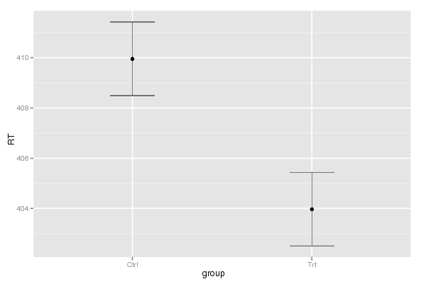
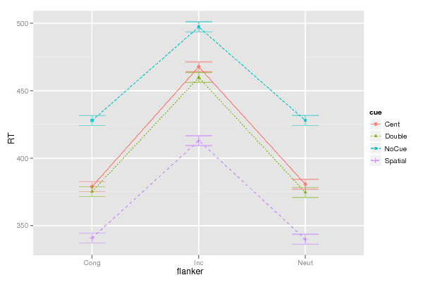
Figures (Output of Computation) | |||||||||||||||||||||||||||||||||||||||||||||||||||||||||||||||||||||||||||||||||||||||||||||||||||||||||||||||||||||||||||||||||||||||||||||||||||||||||||||||||||||||||||||||||||||||||||||||||||||||||||||||||||||||||||||||||||||||||||||||||||||||||||||||||||||||||||||||||||||||||||||||||||||||||||||||||||||||||||||||||||||||||||||||||||||||||||||||||||||||||||||||||||||||||||||||||||||||||||||||||||||||||||||||||||||||||||||||||||||||||||||||||||||||||||||||||||||||||||||||||||||||||||||||||||||||||||||||||||||||||||||||||||||||||||||
Input Parameters & R Code | |||||||||||||||||||||||||||||||||||||||||||||||||||||||||||||||||||||||||||||||||||||||||||||||||||||||||||||||||||||||||||||||||||||||||||||||||||||||||||||||||||||||||||||||||||||||||||||||||||||||||||||||||||||||||||||||||||||||||||||||||||||||||||||||||||||||||||||||||||||||||||||||||||||||||||||||||||||||||||||||||||||||||||||||||||||||||||||||||||||||||||||||||||||||||||||||||||||||||||||||||||||||||||||||||||||||||||||||||||||||||||||||||||||||||||||||||||||||||||||||||||||||||||||||||||||||||||||||||||||||||||||||||||||||||||||
| Parameters (Session): | |||||||||||||||||||||||||||||||||||||||||||||||||||||||||||||||||||||||||||||||||||||||||||||||||||||||||||||||||||||||||||||||||||||||||||||||||||||||||||||||||||||||||||||||||||||||||||||||||||||||||||||||||||||||||||||||||||||||||||||||||||||||||||||||||||||||||||||||||||||||||||||||||||||||||||||||||||||||||||||||||||||||||||||||||||||||||||||||||||||||||||||||||||||||||||||||||||||||||||||||||||||||||||||||||||||||||||||||||||||||||||||||||||||||||||||||||||||||||||||||||||||||||||||||||||||||||||||||||||||||||||||||||||||||||||||
| par1 = 5 ; par2 = 3 ; par3 = 4 ; par4 = 2 ; par5 = 1 ; | |||||||||||||||||||||||||||||||||||||||||||||||||||||||||||||||||||||||||||||||||||||||||||||||||||||||||||||||||||||||||||||||||||||||||||||||||||||||||||||||||||||||||||||||||||||||||||||||||||||||||||||||||||||||||||||||||||||||||||||||||||||||||||||||||||||||||||||||||||||||||||||||||||||||||||||||||||||||||||||||||||||||||||||||||||||||||||||||||||||||||||||||||||||||||||||||||||||||||||||||||||||||||||||||||||||||||||||||||||||||||||||||||||||||||||||||||||||||||||||||||||||||||||||||||||||||||||||||||||||||||||||||||||||||||||||
| Parameters (R input): | |||||||||||||||||||||||||||||||||||||||||||||||||||||||||||||||||||||||||||||||||||||||||||||||||||||||||||||||||||||||||||||||||||||||||||||||||||||||||||||||||||||||||||||||||||||||||||||||||||||||||||||||||||||||||||||||||||||||||||||||||||||||||||||||||||||||||||||||||||||||||||||||||||||||||||||||||||||||||||||||||||||||||||||||||||||||||||||||||||||||||||||||||||||||||||||||||||||||||||||||||||||||||||||||||||||||||||||||||||||||||||||||||||||||||||||||||||||||||||||||||||||||||||||||||||||||||||||||||||||||||||||||||||||||||||||
| par1 = 5 ; par2 = 3 ; par3 = 4 ; par4 = 2 ; par5 = 1 ; | |||||||||||||||||||||||||||||||||||||||||||||||||||||||||||||||||||||||||||||||||||||||||||||||||||||||||||||||||||||||||||||||||||||||||||||||||||||||||||||||||||||||||||||||||||||||||||||||||||||||||||||||||||||||||||||||||||||||||||||||||||||||||||||||||||||||||||||||||||||||||||||||||||||||||||||||||||||||||||||||||||||||||||||||||||||||||||||||||||||||||||||||||||||||||||||||||||||||||||||||||||||||||||||||||||||||||||||||||||||||||||||||||||||||||||||||||||||||||||||||||||||||||||||||||||||||||||||||||||||||||||||||||||||||||||||
| R code (references can be found in the software module): | |||||||||||||||||||||||||||||||||||||||||||||||||||||||||||||||||||||||||||||||||||||||||||||||||||||||||||||||||||||||||||||||||||||||||||||||||||||||||||||||||||||||||||||||||||||||||||||||||||||||||||||||||||||||||||||||||||||||||||||||||||||||||||||||||||||||||||||||||||||||||||||||||||||||||||||||||||||||||||||||||||||||||||||||||||||||||||||||||||||||||||||||||||||||||||||||||||||||||||||||||||||||||||||||||||||||||||||||||||||||||||||||||||||||||||||||||||||||||||||||||||||||||||||||||||||||||||||||||||||||||||||||||||||||||||||
cat1 <- as.numeric(par1) # | |||||||||||||||||||||||||||||||||||||||||||||||||||||||||||||||||||||||||||||||||||||||||||||||||||||||||||||||||||||||||||||||||||||||||||||||||||||||||||||||||||||||||||||||||||||||||||||||||||||||||||||||||||||||||||||||||||||||||||||||||||||||||||||||||||||||||||||||||||||||||||||||||||||||||||||||||||||||||||||||||||||||||||||||||||||||||||||||||||||||||||||||||||||||||||||||||||||||||||||||||||||||||||||||||||||||||||||||||||||||||||||||||||||||||||||||||||||||||||||||||||||||||||||||||||||||||||||||||||||||||||||||||||||||||||||