Free Statistics
of Irreproducible Research!
Description of Statistical Computation | |||||||||||||||||||||
|---|---|---|---|---|---|---|---|---|---|---|---|---|---|---|---|---|---|---|---|---|---|
| Author's title | |||||||||||||||||||||
| Author | *Unverified author* | ||||||||||||||||||||
| R Software Module | rwasp_meanplot.wasp | ||||||||||||||||||||
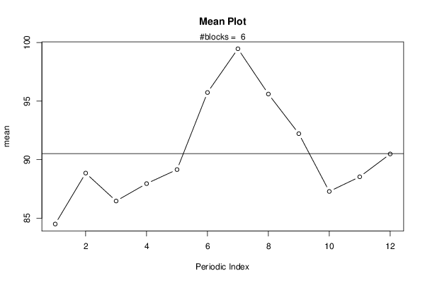
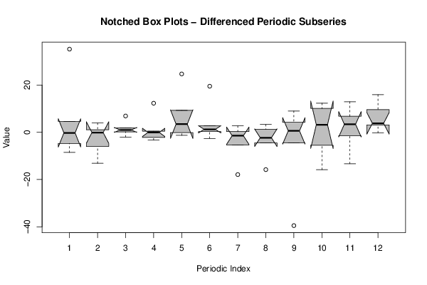
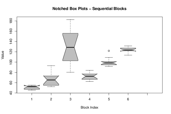
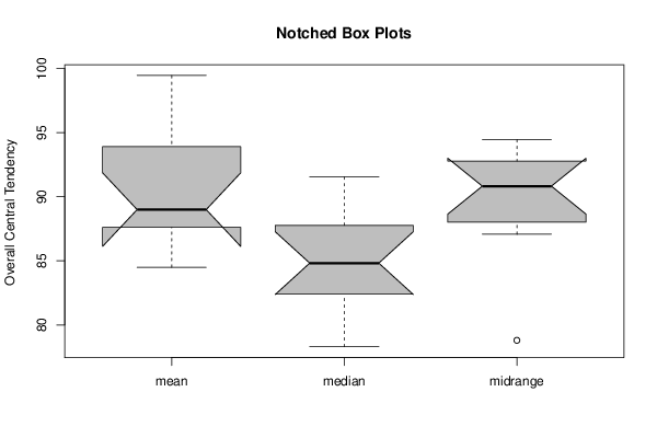
| Title produced by software | Mean Plot | ||||||||||||||||||||
| Date of computation | Sun, 30 Dec 2012 09:14:54 -0500 | ||||||||||||||||||||
| Cite this page as follows | Statistical Computations at FreeStatistics.org, Office for Research Development and Education, URL https://freestatistics.org/blog/index.php?v=date/2012/Dec/30/t1356877072fayzix6yarlz418.htm/, Retrieved Wed, 13 May 2026 14:50:58 +0000 | ||||||||||||||||||||
| Statistical Computations at FreeStatistics.org, Office for Research Development and Education, URL https://freestatistics.org/blog/index.php?pk=204950, Retrieved Wed, 13 May 2026 14:50:58 +0000 | |||||||||||||||||||||
| QR Codes: | |||||||||||||||||||||
|
| |||||||||||||||||||||
| Original text written by user: | |||||||||||||||||||||
| IsPrivate? | No (this computation is public) | ||||||||||||||||||||
| User-defined keywords | |||||||||||||||||||||
| Estimated Impact | 488 | ||||||||||||||||||||
Tree of Dependent Computations | |||||||||||||||||||||
| Family? (F = Feedback message, R = changed R code, M = changed R Module, P = changed Parameters, D = changed Data) | |||||||||||||||||||||
| - [Mean Plot] [Mean plot eigen r...] [2012-12-27 11:32:26] [270271722390d2035805c3d10dfa13a8] - R PD [Mean Plot] [Mean plot eigen r...] [2012-12-30 14:14:54] [56be9a844975c6d0d36e88eaea5fb75b] [Current] | |||||||||||||||||||||
| Feedback Forum | |||||||||||||||||||||
Post a new message | |||||||||||||||||||||
Dataset | |||||||||||||||||||||
| Dataseries X: | |||||||||||||||||||||
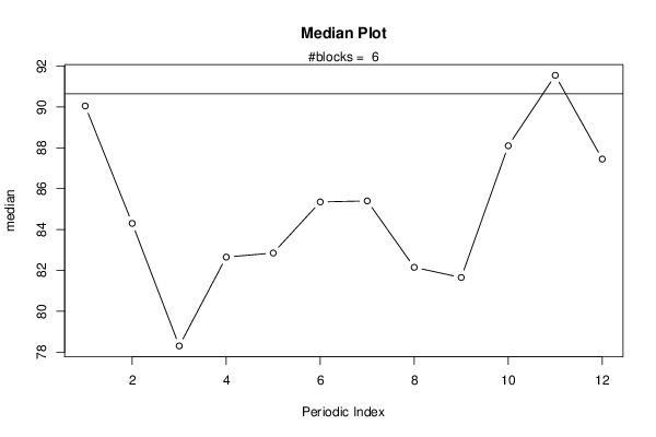
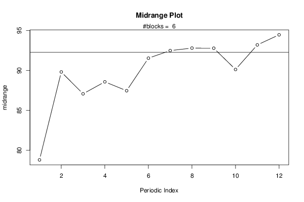
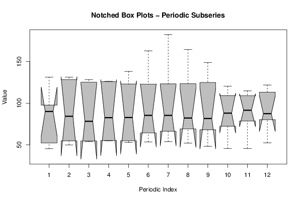
45.3 49.9 53.8 55.1 52.9 53.5 53.8 52 48.2 45.5 45.7 52.5 52.3 54.8 54.7 54.9 54.9 64.2 66.4 69.1 68.3 77.3 89.6 93 96.1 131.3 125.3 126 138.3 163 182.5 164.6 148.8 109.3 93.5 80.2 84 75.5 62.4 64.2 64.7 71 73.7 72.6 68.1 72.3 78.5 81.9 97.8 93.1 94.2 101.1 101 99.7 97.1 91.7 95 98.9 109 121.9 131.5 128.5 128.4 126.4 123.1 123 123.3 123.6 124.9 120.4 114.9 113.4 | |||||||||||||||||||||
Tables (Output of Computation) | |||||||||||||||||||||
| |||||||||||||||||||||
Figures (Output of Computation) | |||||||||||||||||||||
Input Parameters & R Code | |||||||||||||||||||||
| Parameters (Session): | |||||||||||||||||||||
| par1 = 12 ; | |||||||||||||||||||||
| Parameters (R input): | |||||||||||||||||||||
| par1 = 12 ; | |||||||||||||||||||||
| R code (references can be found in the software module): | |||||||||||||||||||||
par1 <- as.numeric(par1) | |||||||||||||||||||||