Repository of Reproducible Computations

Free Statistics

of Irreproducible Research!

Author's title

Author

*The author of this computation has been verified*

R Software Module

rwasp_autocorrelation.wasp

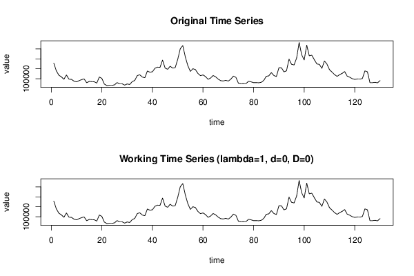
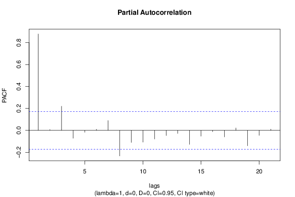
Title produced by software

(Partial) Autocorrelation Function

Date of computation

Mon, 03 Dec 2012 14:55:49 -0500

Cite this page as follows

Statistical Computations at FreeStatistics.org, Office for Research Development and Education, URL https://freestatistics.org/blog/index.php?v=date/2012/Dec/03/t1354564573qlyh908ov05meef.htm/, Retrieved Sun, 28 Apr 2024 06:53:14 +0000

Statistical Computations at FreeStatistics.org, Office for Research Development and Education, URL https://freestatistics.org/blog/index.php?pk=195994, Retrieved Sun, 28 Apr 2024 06:53:14 +0000

QR Codes:

Paste this QR Code to cite your computation.

Original text written by user:

IsPrivate?

No (this computation is public)

User-defined keywords

Estimated Impact

Family? (F = Feedback message, R = changed R code, M = changed R Module, P = changed Parameters, D = changed Data)

-       [(Partial) Autocorrelation Function] [Workshop 9 - auto...] [2012-12-03 19:55:49] [729cfeb7382ca95684eaaf6b24800101] [Current]
- R P     [(Partial) Autocorrelation Function] [Workshop 9 - auto...] [2012-12-03 19:57:39] [c85dbc843174c8f40de92b1c92b5205a] 
-   P       [(Partial) Autocorrelation Function] [Workshop 9 - auto...] [2012-12-03 19:59:54] [c85dbc843174c8f40de92b1c92b5205a] 
- RMP       [Spectral Analysis] [Workshop 9 - peri...] [2012-12-03 20:02:49] [c85dbc843174c8f40de92b1c92b5205a] 
- R P         [Spectral Analysis] [Workshop 9 - peri...] [2012-12-03 20:04:57] [c85dbc843174c8f40de92b1c92b5205a] 
- RMP           [Variance Reduction Matrix] [Workshop 9 - vari...] [2012-12-03 20:17:14] [c85dbc843174c8f40de92b1c92b5205a] 
- RMP           [Standard Deviation-Mean Plot] [Workshop 9 - mean...] [2012-12-03 20:19:24] [c85dbc843174c8f40de92b1c92b5205a] 
- RMP           [ARIMA Backward Selection] [Workshop 9 - ARIM...] [2012-12-03 20:32:52] [c85dbc843174c8f40de92b1c92b5205a] 
-   P             [ARIMA Backward Selection] [Workshop 9 - ARIM...] [2012-12-04 11:24:44] [c85dbc843174c8f40de92b1c92b5205a] 
- RMP             [Skewness and Kurtosis Test] [Workshop 9 - skew...] [2012-12-04 11:43:19] [c85dbc843174c8f40de92b1c92b5205a] 
- RMP             [ARIMA Forecasting] [Workshop 9 - ARIM...] [2012-12-04 11:52:28] [c85dbc843174c8f40de92b1c92b5205a] 

Feedback Forum

Post a new message

Dataseries X:

Download CSV

Histogram

Boxplots

Summary of computational transaction
Raw Input	view raw input (R code)
Raw Output	view raw output of R engine
Computing time	2 seconds
R Server	'Gwilym Jenkins' @ jenkins.wessa.net

\begin{tabular}{lllllllll}
\hline
Summary of computational transaction \tabularnewline
Raw Input & view raw input (R code)  \tabularnewline
Raw Output & view raw output of R engine  \tabularnewline
Computing time & 2 seconds \tabularnewline
R Server & 'Gwilym Jenkins' @ jenkins.wessa.net \tabularnewline
\hline
\end{tabular}
%Source: https://freestatistics.org/blog/index.php?pk=195994&T=0

[TABLE]
[ROW][C]Summary of computational transaction[/C][/ROW]
[ROW][C]Raw Input[/C][C]view raw input (R code) [/C][/ROW]
[ROW][C]Raw Output[/C][C]view raw output of R engine [/C][/ROW]
[ROW][C]Computing time[/C][C]2 seconds[/C][/ROW]
[ROW][C]R Server[/C][C]'Gwilym Jenkins' @ jenkins.wessa.net[/C][/ROW]
[/TABLE]
Source: https://freestatistics.org/blog/index.php?pk=195994&T=0

Globally Unique Identifier (entire table): ba.freestatistics.org/blog/index.php?pk=195994&T=0

As an alternative you can also use a QR Code:

The GUIDs for individual cells are displayed in the table below:

Summary of computational transaction
Raw Input	view raw input (R code)
Raw Output	view raw output of R engine
Computing time	2 seconds
R Server	'Gwilym Jenkins' @ jenkins.wessa.net

Autocorrelation Function
Time lag k	ACF(k)	T-STAT	P-value
1	0.878676	10.0184	0
2	0.773772	8.8224	0
3	0.731548	8.3409	0
4	0.671828	7.66	0
5	0.602558	6.8702	0
6	0.551183	6.2845	0
7	0.525735	5.9943	0
8	0.445154	5.0755	1e-06
9	0.346336	3.9488	6.4e-05
10	0.267445	3.0493	0.00139
11	0.187637	2.1394	0.017136
12	0.108587	1.2381	0.108959
13	0.041056	0.4681	0.320246
14	-0.030156	-0.3438	0.365765
15	-0.105935	-1.2078	0.11465
16	-0.169957	-1.9378	0.027407
17	-0.232647	-2.6526	0.004492
18	-0.282305	-3.2188	0.000813
19	-0.345793	-3.9426	6.6e-05
20	-0.400579	-4.5673	6e-06
21	-0.430799	-4.9119	1e-06

\begin{tabular}{lllllllll}
\hline
Autocorrelation Function \tabularnewline
Time lag k & ACF(k) & T-STAT & P-value \tabularnewline
1 & 0.878676 & 10.0184 & 0 \tabularnewline
2 & 0.773772 & 8.8224 & 0 \tabularnewline
3 & 0.731548 & 8.3409 & 0 \tabularnewline
4 & 0.671828 & 7.66 & 0 \tabularnewline
5 & 0.602558 & 6.8702 & 0 \tabularnewline
6 & 0.551183 & 6.2845 & 0 \tabularnewline
7 & 0.525735 & 5.9943 & 0 \tabularnewline
8 & 0.445154 & 5.0755 & 1e-06 \tabularnewline
9 & 0.346336 & 3.9488 & 6.4e-05 \tabularnewline
10 & 0.267445 & 3.0493 & 0.00139 \tabularnewline
11 & 0.187637 & 2.1394 & 0.017136 \tabularnewline
12 & 0.108587 & 1.2381 & 0.108959 \tabularnewline
13 & 0.041056 & 0.4681 & 0.320246 \tabularnewline
14 & -0.030156 & -0.3438 & 0.365765 \tabularnewline
15 & -0.105935 & -1.2078 & 0.11465 \tabularnewline
16 & -0.169957 & -1.9378 & 0.027407 \tabularnewline
17 & -0.232647 & -2.6526 & 0.004492 \tabularnewline
18 & -0.282305 & -3.2188 & 0.000813 \tabularnewline
19 & -0.345793 & -3.9426 & 6.6e-05 \tabularnewline
20 & -0.400579 & -4.5673 & 6e-06 \tabularnewline
21 & -0.430799 & -4.9119 & 1e-06 \tabularnewline
\hline
\end{tabular}
%Source: https://freestatistics.org/blog/index.php?pk=195994&T=1

[TABLE]
[ROW][C]Autocorrelation Function[/C][/ROW]
[ROW][C]Time lag k[/C][C]ACF(k)[/C][C]T-STAT[/C][C]P-value[/C][/ROW]
[ROW][C]1[/C][C]0.878676[/C][C]10.0184[/C][C]0[/C][/ROW]
[ROW][C]2[/C][C]0.773772[/C][C]8.8224[/C][C]0[/C][/ROW]
[ROW][C]3[/C][C]0.731548[/C][C]8.3409[/C][C]0[/C][/ROW]
[ROW][C]4[/C][C]0.671828[/C][C]7.66[/C][C]0[/C][/ROW]
[ROW][C]5[/C][C]0.602558[/C][C]6.8702[/C][C]0[/C][/ROW]
[ROW][C]6[/C][C]0.551183[/C][C]6.2845[/C][C]0[/C][/ROW]
[ROW][C]7[/C][C]0.525735[/C][C]5.9943[/C][C]0[/C][/ROW]
[ROW][C]8[/C][C]0.445154[/C][C]5.0755[/C][C]1e-06[/C][/ROW]
[ROW][C]9[/C][C]0.346336[/C][C]3.9488[/C][C]6.4e-05[/C][/ROW]
[ROW][C]10[/C][C]0.267445[/C][C]3.0493[/C][C]0.00139[/C][/ROW]
[ROW][C]11[/C][C]0.187637[/C][C]2.1394[/C][C]0.017136[/C][/ROW]
[ROW][C]12[/C][C]0.108587[/C][C]1.2381[/C][C]0.108959[/C][/ROW]
[ROW][C]13[/C][C]0.041056[/C][C]0.4681[/C][C]0.320246[/C][/ROW]
[ROW][C]14[/C][C]-0.030156[/C][C]-0.3438[/C][C]0.365765[/C][/ROW]
[ROW][C]15[/C][C]-0.105935[/C][C]-1.2078[/C][C]0.11465[/C][/ROW]
[ROW][C]16[/C][C]-0.169957[/C][C]-1.9378[/C][C]0.027407[/C][/ROW]
[ROW][C]17[/C][C]-0.232647[/C][C]-2.6526[/C][C]0.004492[/C][/ROW]
[ROW][C]18[/C][C]-0.282305[/C][C]-3.2188[/C][C]0.000813[/C][/ROW]
[ROW][C]19[/C][C]-0.345793[/C][C]-3.9426[/C][C]6.6e-05[/C][/ROW]
[ROW][C]20[/C][C]-0.400579[/C][C]-4.5673[/C][C]6e-06[/C][/ROW]
[ROW][C]21[/C][C]-0.430799[/C][C]-4.9119[/C][C]1e-06[/C][/ROW]
[/TABLE]
Source: https://freestatistics.org/blog/index.php?pk=195994&T=1

Globally Unique Identifier (entire table): ba.freestatistics.org/blog/index.php?pk=195994&T=1

As an alternative you can also use a QR Code:

The GUIDs for individual cells are displayed in the table below:

Autocorrelation Function
Time lag k	ACF(k)	T-STAT	P-value
1	0.878676	10.0184	0
2	0.773772	8.8224	0
3	0.731548	8.3409	0
4	0.671828	7.66	0
5	0.602558	6.8702	0
6	0.551183	6.2845	0
7	0.525735	5.9943	0
8	0.445154	5.0755	1e-06
9	0.346336	3.9488	6.4e-05
10	0.267445	3.0493	0.00139
11	0.187637	2.1394	0.017136
12	0.108587	1.2381	0.108959
13	0.041056	0.4681	0.320246
14	-0.030156	-0.3438	0.365765
15	-0.105935	-1.2078	0.11465
16	-0.169957	-1.9378	0.027407
17	-0.232647	-2.6526	0.004492
18	-0.282305	-3.2188	0.000813
19	-0.345793	-3.9426	6.6e-05
20	-0.400579	-4.5673	6e-06
21	-0.430799	-4.9119	1e-06

Partial Autocorrelation Function
Time lag k	PACF(k)	T-STAT	P-value
1	0.878676	10.0184	0
2	0.007462	0.0851	0.466163
3	0.220123	2.5098	0.006654
4	-0.071996	-0.8209	0.206608
5	-0.017427	-0.1987	0.421405
6	0.010038	0.1145	0.454526
7	0.089851	1.0245	0.153762
8	-0.233055	-2.6572	0.004433
9	-0.109768	-1.2515	0.106492
10	-0.107408	-1.2246	0.111462
11	-0.078332	-0.8931	0.186722
12	-0.046905	-0.5348	0.296853
13	-0.027945	-0.3186	0.375261
14	-0.127687	-1.4559	0.073922
15	-0.052745	-0.6014	0.274317
16	-0.012024	-0.1371	0.445585
17	-0.059702	-0.6807	0.248634
18	0.021754	0.248	0.40225
19	-0.140395	-1.6007	0.05593
20	-0.045599	-0.5199	0.302007
21	0.011408	0.1301	0.448357

\begin{tabular}{lllllllll}
\hline
Partial Autocorrelation Function \tabularnewline
Time lag k & PACF(k) & T-STAT & P-value \tabularnewline
1 & 0.878676 & 10.0184 & 0 \tabularnewline
2 & 0.007462 & 0.0851 & 0.466163 \tabularnewline
3 & 0.220123 & 2.5098 & 0.006654 \tabularnewline
4 & -0.071996 & -0.8209 & 0.206608 \tabularnewline
5 & -0.017427 & -0.1987 & 0.421405 \tabularnewline
6 & 0.010038 & 0.1145 & 0.454526 \tabularnewline
7 & 0.089851 & 1.0245 & 0.153762 \tabularnewline
8 & -0.233055 & -2.6572 & 0.004433 \tabularnewline
9 & -0.109768 & -1.2515 & 0.106492 \tabularnewline
10 & -0.107408 & -1.2246 & 0.111462 \tabularnewline
11 & -0.078332 & -0.8931 & 0.186722 \tabularnewline
12 & -0.046905 & -0.5348 & 0.296853 \tabularnewline
13 & -0.027945 & -0.3186 & 0.375261 \tabularnewline
14 & -0.127687 & -1.4559 & 0.073922 \tabularnewline
15 & -0.052745 & -0.6014 & 0.274317 \tabularnewline
16 & -0.012024 & -0.1371 & 0.445585 \tabularnewline
17 & -0.059702 & -0.6807 & 0.248634 \tabularnewline
18 & 0.021754 & 0.248 & 0.40225 \tabularnewline
19 & -0.140395 & -1.6007 & 0.05593 \tabularnewline
20 & -0.045599 & -0.5199 & 0.302007 \tabularnewline
21 & 0.011408 & 0.1301 & 0.448357 \tabularnewline
\hline
\end{tabular}
%Source: https://freestatistics.org/blog/index.php?pk=195994&T=2

[TABLE]
[ROW][C]Partial Autocorrelation Function[/C][/ROW]
[ROW][C]Time lag k[/C][C]PACF(k)[/C][C]T-STAT[/C][C]P-value[/C][/ROW]
[ROW][C]1[/C][C]0.878676[/C][C]10.0184[/C][C]0[/C][/ROW]
[ROW][C]2[/C][C]0.007462[/C][C]0.0851[/C][C]0.466163[/C][/ROW]
[ROW][C]3[/C][C]0.220123[/C][C]2.5098[/C][C]0.006654[/C][/ROW]
[ROW][C]4[/C][C]-0.071996[/C][C]-0.8209[/C][C]0.206608[/C][/ROW]
[ROW][C]5[/C][C]-0.017427[/C][C]-0.1987[/C][C]0.421405[/C][/ROW]
[ROW][C]6[/C][C]0.010038[/C][C]0.1145[/C][C]0.454526[/C][/ROW]
[ROW][C]7[/C][C]0.089851[/C][C]1.0245[/C][C]0.153762[/C][/ROW]
[ROW][C]8[/C][C]-0.233055[/C][C]-2.6572[/C][C]0.004433[/C][/ROW]
[ROW][C]9[/C][C]-0.109768[/C][C]-1.2515[/C][C]0.106492[/C][/ROW]
[ROW][C]10[/C][C]-0.107408[/C][C]-1.2246[/C][C]0.111462[/C][/ROW]
[ROW][C]11[/C][C]-0.078332[/C][C]-0.8931[/C][C]0.186722[/C][/ROW]
[ROW][C]12[/C][C]-0.046905[/C][C]-0.5348[/C][C]0.296853[/C][/ROW]
[ROW][C]13[/C][C]-0.027945[/C][C]-0.3186[/C][C]0.375261[/C][/ROW]
[ROW][C]14[/C][C]-0.127687[/C][C]-1.4559[/C][C]0.073922[/C][/ROW]
[ROW][C]15[/C][C]-0.052745[/C][C]-0.6014[/C][C]0.274317[/C][/ROW]
[ROW][C]16[/C][C]-0.012024[/C][C]-0.1371[/C][C]0.445585[/C][/ROW]
[ROW][C]17[/C][C]-0.059702[/C][C]-0.6807[/C][C]0.248634[/C][/ROW]
[ROW][C]18[/C][C]0.021754[/C][C]0.248[/C][C]0.40225[/C][/ROW]
[ROW][C]19[/C][C]-0.140395[/C][C]-1.6007[/C][C]0.05593[/C][/ROW]
[ROW][C]20[/C][C]-0.045599[/C][C]-0.5199[/C][C]0.302007[/C][/ROW]
[ROW][C]21[/C][C]0.011408[/C][C]0.1301[/C][C]0.448357[/C][/ROW]
[/TABLE]
Source: https://freestatistics.org/blog/index.php?pk=195994&T=2

Globally Unique Identifier (entire table): ba.freestatistics.org/blog/index.php?pk=195994&T=2

As an alternative you can also use a QR Code:

The GUIDs for individual cells are displayed in the table below:

Partial Autocorrelation Function
Time lag k	PACF(k)	T-STAT	P-value
1	0.878676	10.0184	0
2	0.007462	0.0851	0.466163
3	0.220123	2.5098	0.006654
4	-0.071996	-0.8209	0.206608
5	-0.017427	-0.1987	0.421405
6	0.010038	0.1145	0.454526
7	0.089851	1.0245	0.153762
8	-0.233055	-2.6572	0.004433
9	-0.109768	-1.2515	0.106492
10	-0.107408	-1.2246	0.111462
11	-0.078332	-0.8931	0.186722
12	-0.046905	-0.5348	0.296853
13	-0.027945	-0.3186	0.375261
14	-0.127687	-1.4559	0.073922
15	-0.052745	-0.6014	0.274317
16	-0.012024	-0.1371	0.445585
17	-0.059702	-0.6807	0.248634
18	0.021754	0.248	0.40225
19	-0.140395	-1.6007	0.05593
20	-0.045599	-0.5199	0.302007
21	0.011408	0.1301	0.448357

Figure 1

PNG link

Postscript link

PDF link

Figure 2

PNG link

Postscript link

PDF link

Figure 3

PNG link

Postscript link

PDF link

Parameters (Session):

par1 = Default ; par2 = 1 ; par3 = 0 ; par4 = 0 ; par5 = 4 ; par6 = White Noise ; par7 = 0.95 ;

Parameters (R input):

par1 = Default ; par2 = 1 ; par3 = 0 ; par4 = 0 ; par5 = 4 ; par6 = White Noise ; par7 = 0.95 ; par8 = ;

R code (references can be found in the software module):

if (par1 == 'Default') {
par1 = 10*log10(length(x))
} else {
par1 <- as.numeric(par1)
}
par2 <- as.numeric(par2)
par3 <- as.numeric(par3)
par4 <- as.numeric(par4)
par5 <- as.numeric(par5)
if (par6 == 'White Noise') par6 <- 'white' else par6 <- 'ma'
par7 <- as.numeric(par7)
if (par8 != '') par8 <- as.numeric(par8)
ox <- x
if (par8 == '') {
if (par2 == 0) {
x <- log(x)
} else {
x <- (x ^ par2 - 1) / par2
}
} else {
x <- log(x,base=par8)
}
if (par3 > 0) x <- diff(x,lag=1,difference=par3)
if (par4 > 0) x <- diff(x,lag=par5,difference=par4)
bitmap(file='picts.png')
op <- par(mfrow=c(2,1))
plot(ox,type='l',main='Original Time Series',xlab='time',ylab='value')
if (par8=='') {
mytitle <- paste('Working Time Series (lambda=',par2,', d=',par3,', D=',par4,')',sep='')
mysub <- paste('(lambda=',par2,', d=',par3,', D=',par4,', CI=', par7, ', CI type=',par6,')',sep='')
} else {
mytitle <- paste('Working Time Series (base=',par8,', d=',par3,', D=',par4,')',sep='')
mysub <- paste('(base=',par8,', d=',par3,', D=',par4,', CI=', par7, ', CI type=',par6,')',sep='')
}
plot(x,type='l', main=mytitle,xlab='time',ylab='value')
par(op)
dev.off()
bitmap(file='pic1.png')
racf <- acf(x, par1, main='Autocorrelation', xlab='time lag', ylab='ACF', ci.type=par6, ci=par7, sub=mysub)
dev.off()
bitmap(file='pic2.png')
rpacf <- pacf(x,par1,main='Partial Autocorrelation',xlab='lags',ylab='PACF',sub=mysub)
dev.off()
(myacf <- c(racf$acf))
(mypacf <- c(rpacf$acf))
lengthx <- length(x)
sqrtn <- sqrt(lengthx)
load(file='createtable')
a<-table.start()
a<-table.row.start(a)
a<-table.element(a,'Autocorrelation Function',4,TRUE)
a<-table.row.end(a)
a<-table.row.start(a)
a<-table.element(a,'Time lag k',header=TRUE)
a<-table.element(a,hyperlink('basics.htm','ACF(k)','click here for more information about the Autocorrelation Function'),header=TRUE)
a<-table.element(a,'T-STAT',header=TRUE)
a<-table.element(a,'P-value',header=TRUE)
a<-table.row.end(a)
for (i in 2:(par1+1)) {
a<-table.row.start(a)
a<-table.element(a,i-1,header=TRUE)
a<-table.element(a,round(myacf[i],6))
mytstat <- myacf[i]*sqrtn
a<-table.element(a,round(mytstat,4))
a<-table.element(a,round(1-pt(abs(mytstat),lengthx),6))
a<-table.row.end(a)
}
a<-table.end(a)
table.save(a,file='mytable.tab')
a<-table.start()
a<-table.row.start(a)
a<-table.element(a,'Partial Autocorrelation Function',4,TRUE)
a<-table.row.end(a)
a<-table.row.start(a)
a<-table.element(a,'Time lag k',header=TRUE)
a<-table.element(a,hyperlink('basics.htm','PACF(k)','click here for more information about the Partial Autocorrelation Function'),header=TRUE)
a<-table.element(a,'T-STAT',header=TRUE)
a<-table.element(a,'P-value',header=TRUE)
a<-table.row.end(a)
for (i in 1:par1) {
a<-table.row.start(a)
a<-table.element(a,i,header=TRUE)
a<-table.element(a,round(mypacf[i],6))
mytstat <- mypacf[i]*sqrtn
a<-table.element(a,round(mytstat,4))
a<-table.element(a,round(1-pt(abs(mytstat),lengthx),6))
a<-table.row.end(a)
}
a<-table.end(a)
table.save(a,file='mytable1.tab')

Free Statistics

Description of Statistical Computation

Tree of Dependent Computations

Dataset

Tables (Output of Computation)

Figures (Output of Computation)

Input Parameters & R Code