Free Statistics
of Irreproducible Research!
Description of Statistical Computation | |||||||||||||||||||||||||||||||||||||||||||||||||||||||||||||||||||||||||||||||||
|---|---|---|---|---|---|---|---|---|---|---|---|---|---|---|---|---|---|---|---|---|---|---|---|---|---|---|---|---|---|---|---|---|---|---|---|---|---|---|---|---|---|---|---|---|---|---|---|---|---|---|---|---|---|---|---|---|---|---|---|---|---|---|---|---|---|---|---|---|---|---|---|---|---|---|---|---|---|---|---|---|---|
| Author's title | |||||||||||||||||||||||||||||||||||||||||||||||||||||||||||||||||||||||||||||||||
| Author | *Unverified author* | ||||||||||||||||||||||||||||||||||||||||||||||||||||||||||||||||||||||||||||||||
| R Software Module | rwasp_bootstrapplot.wasp | ||||||||||||||||||||||||||||||||||||||||||||||||||||||||||||||||||||||||||||||||
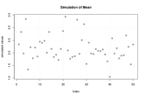
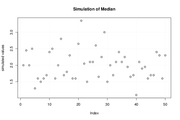
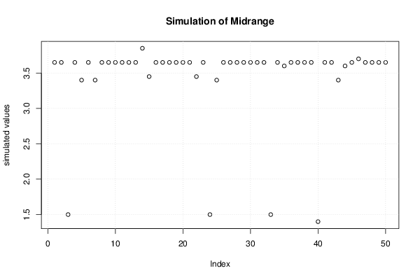
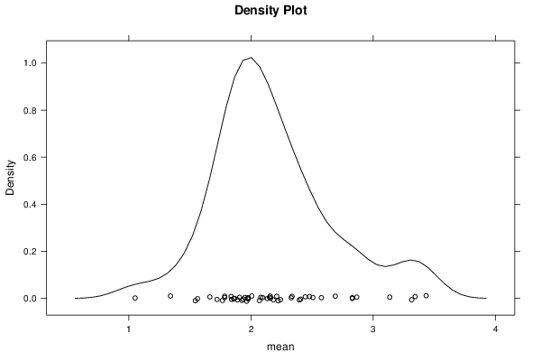
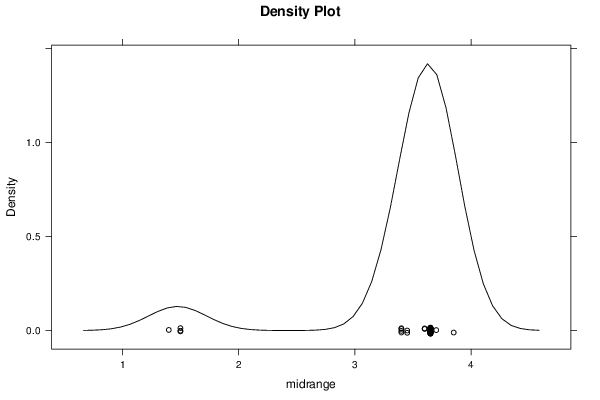
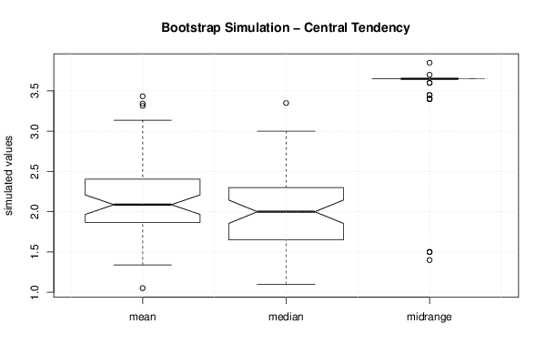
| Title produced by software | Blocked Bootstrap Plot - Central Tendency | ||||||||||||||||||||||||||||||||||||||||||||||||||||||||||||||||||||||||||||||||
| Date of computation | Mon, 03 Dec 2012 14:10:09 -0500 | ||||||||||||||||||||||||||||||||||||||||||||||||||||||||||||||||||||||||||||||||
| Cite this page as follows | Statistical Computations at FreeStatistics.org, Office for Research Development and Education, URL https://freestatistics.org/blog/index.php?v=date/2012/Dec/03/t135456182910yxdu9s5q8wsik.htm/, Retrieved Sun, 28 Apr 2024 15:51:54 +0000 | ||||||||||||||||||||||||||||||||||||||||||||||||||||||||||||||||||||||||||||||||
| Statistical Computations at FreeStatistics.org, Office for Research Development and Education, URL https://freestatistics.org/blog/index.php?pk=195957, Retrieved Sun, 28 Apr 2024 15:51:54 +0000 | |||||||||||||||||||||||||||||||||||||||||||||||||||||||||||||||||||||||||||||||||
| QR Codes: | |||||||||||||||||||||||||||||||||||||||||||||||||||||||||||||||||||||||||||||||||
|
| |||||||||||||||||||||||||||||||||||||||||||||||||||||||||||||||||||||||||||||||||
| Original text written by user: | |||||||||||||||||||||||||||||||||||||||||||||||||||||||||||||||||||||||||||||||||
| IsPrivate? | No (this computation is public) | ||||||||||||||||||||||||||||||||||||||||||||||||||||||||||||||||||||||||||||||||
| User-defined keywords | |||||||||||||||||||||||||||||||||||||||||||||||||||||||||||||||||||||||||||||||||
| Estimated Impact | 137 | ||||||||||||||||||||||||||||||||||||||||||||||||||||||||||||||||||||||||||||||||
Tree of Dependent Computations | |||||||||||||||||||||||||||||||||||||||||||||||||||||||||||||||||||||||||||||||||
| Family? (F = Feedback message, R = changed R code, M = changed R Module, P = changed Parameters, D = changed Data) | |||||||||||||||||||||||||||||||||||||||||||||||||||||||||||||||||||||||||||||||||
| - [Blocked Bootstrap Plot - Central Tendency] [] [2012-12-03 19:10:09] [19a5fa3cc9952272699ac0aa748608b8] [Current] - RMPD [Variability] [] [2012-12-09 15:39:32] [73ff502f5cc0e8f9d4cad04b672b43dc] - RMPD [Standard Deviation Plot] [] [2012-12-09 16:04:26] [73ff502f5cc0e8f9d4cad04b672b43dc] - RMPD [Standard Deviation-Mean Plot] [] [2012-12-09 17:36:52] [73ff502f5cc0e8f9d4cad04b672b43dc] - RMPD [Classical Decomposition] [] [2012-12-09 17:45:19] [73ff502f5cc0e8f9d4cad04b672b43dc] | |||||||||||||||||||||||||||||||||||||||||||||||||||||||||||||||||||||||||||||||||
| Feedback Forum | |||||||||||||||||||||||||||||||||||||||||||||||||||||||||||||||||||||||||||||||||
Post a new message | |||||||||||||||||||||||||||||||||||||||||||||||||||||||||||||||||||||||||||||||||
Dataset | |||||||||||||||||||||||||||||||||||||||||||||||||||||||||||||||||||||||||||||||||
| Dataseries X: | |||||||||||||||||||||||||||||||||||||||||||||||||||||||||||||||||||||||||||||||||
1,6 2 2,6 3 2,6 2,9 2,5 2,4 1,5 1,1 0,6 0,9 1,1 1,5 1,7 1,2 0,4 -0,7 -1,4 -1,6 -1,2 -0,4 -0,2 -0,3 -0,5 0 -0,5 0,2 0,7 1,6 2,6 3,3 3,3 3,2 3,5 3,9 4,5 4,6 6,6 7,1 8,9 8,8 8,5 7,6 7,5 7,5 6,1 6,3 8,4 7,1 5,6 4,2 2,1 1,2 0,9 1,4 1,7 1,7 1,9 1,3 -0,7 0,3 0,8 0,9 1,1 2,5 2,7 3,3 4,2 3,8 3,8 3,2 2,9 1,9 1,7 1,6 1,7 1,2 0,7 -0,2 -1,5 -1,2 -1 0 -0,6 0,7 1,3 0,8 1 0,5 0,3 1 1 1,1 1,5 1,5 2 1,7 0,6 1,2 1,5 2,1 3,2 3,9 4,6 4,2 4,4 3,7 3,7 2,8 2,9 3,9 3,1 3 2,8 2,4 2,1 3,1 3 3,1 3,3 3,3 3,8 3,1 3,9 4 4,4 3,7 3,6 3,4 2,8 2,8 2,6 3,3 2,4 1,6 0,7 0 -1,1 -1,2 -1,3 -1,6 -1,3 -1,6 -1,1 -1 0,3 1,2 0,7 1,1 2,1 2,5 2,3 2,3 2,6 3,2 2,2 2,7 2,2 1,4 2,4 2 1,3 1,1 1,4 1,8 1,9 1,6 | |||||||||||||||||||||||||||||||||||||||||||||||||||||||||||||||||||||||||||||||||
Tables (Output of Computation) | |||||||||||||||||||||||||||||||||||||||||||||||||||||||||||||||||||||||||||||||||
| |||||||||||||||||||||||||||||||||||||||||||||||||||||||||||||||||||||||||||||||||
Figures (Output of Computation) | |||||||||||||||||||||||||||||||||||||||||||||||||||||||||||||||||||||||||||||||||
Input Parameters & R Code | |||||||||||||||||||||||||||||||||||||||||||||||||||||||||||||||||||||||||||||||||
| Parameters (Session): | |||||||||||||||||||||||||||||||||||||||||||||||||||||||||||||||||||||||||||||||||
| par1 = 750 ; par2 = 5 ; par3 = 0 ; | |||||||||||||||||||||||||||||||||||||||||||||||||||||||||||||||||||||||||||||||||
| Parameters (R input): | |||||||||||||||||||||||||||||||||||||||||||||||||||||||||||||||||||||||||||||||||
| par1 = 50 ; par2 = 12 ; | |||||||||||||||||||||||||||||||||||||||||||||||||||||||||||||||||||||||||||||||||
| R code (references can be found in the software module): | |||||||||||||||||||||||||||||||||||||||||||||||||||||||||||||||||||||||||||||||||
par1 <- as.numeric(par1) | |||||||||||||||||||||||||||||||||||||||||||||||||||||||||||||||||||||||||||||||||