Repository of Reproducible Computations

Free Statistics

of Irreproducible Research!

Author's title

Author

*Unverified author*

R Software Module

rwasp_autocorrelation.wasp

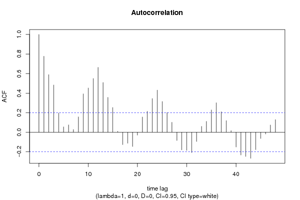
Title produced by software

(Partial) Autocorrelation Function

Date of computation

Thu, 19 May 2011 07:06:18 +0000

Cite this page as follows

Statistical Computations at FreeStatistics.org, Office for Research Development and Education, URL https://freestatistics.org/blog/index.php?v=date/2011/May/19/t1305788572xsx0kynzsq6wj22.htm/, Retrieved Sun, 05 May 2024 03:43:47 +0000

Statistical Computations at FreeStatistics.org, Office for Research Development and Education, URL https://freestatistics.org/blog/index.php?pk=121946, Retrieved Sun, 05 May 2024 03:43:47 +0000

QR Codes:

Paste this QR Code to cite your computation.

Original text written by user:

IsPrivate?

No (this computation is public)

User-defined keywords

KDGP2W12

Estimated Impact

142

Family? (F = Feedback message, R = changed R code, M = changed R Module, P = changed Parameters, D = changed Data)

-     [(Partial) Autocorrelation Function] [De inschrijving v...] [2010-11-23 22:10:09] [3e532679ec753acf7892d78d91c458c8]
- R PD    [(Partial) Autocorrelation Function] [autocorrelatie US...] [2011-05-19 07:06:18] [a84eb6f3c59b92a1a531ce943c0523d4] [Current]
- R P       [(Partial) Autocorrelation Function] [autocorrelatie se...] [2011-05-19 07:09:01] [d460d5fbfa759ad1669bb34c73f51f31] 
- RMPD      [Bootstrap Plot - Central Tendency] [Bootstrap Plot Ma...] [2011-05-19 07:13:05] [d460d5fbfa759ad1669bb34c73f51f31] 
- RMP       [Blocked Bootstrap Plot - Central Tendency] [bootstrap plot US...] [2011-05-19 07:20:03] [d460d5fbfa759ad1669bb34c73f51f31] 
- RMPD      [Variability] [spreidingsmaten S...] [2011-05-19 07:26:19] [d460d5fbfa759ad1669bb34c73f51f31] 
- RMPD      [Standard Deviation Plot] [Standard Deviatio...] [2011-05-19 07:29:06] [d460d5fbfa759ad1669bb34c73f51f31] 

Feedback Forum

Post a new message

Dataseries X:

Download CSV

Histogram

Boxplots

Summary of computational transaction
Raw Input	view raw input (R code)
Raw Output	view raw output of R engine
Computing time	2 seconds
R Server	'Sir Ronald Aylmer Fisher' @ 193.190.124.24

\begin{tabular}{lllllllll}
\hline
Summary of computational transaction \tabularnewline
Raw Input & view raw input (R code)  \tabularnewline
Raw Output & view raw output of R engine  \tabularnewline
Computing time & 2 seconds \tabularnewline
R Server & 'Sir Ronald Aylmer Fisher' @ 193.190.124.24 \tabularnewline
\hline
\end{tabular}
%Source: https://freestatistics.org/blog/index.php?pk=121946&T=0

[TABLE]
[ROW][C]Summary of computational transaction[/C][/ROW]
[ROW][C]Raw Input[/C][C]view raw input (R code) [/C][/ROW]
[ROW][C]Raw Output[/C][C]view raw output of R engine [/C][/ROW]
[ROW][C]Computing time[/C][C]2 seconds[/C][/ROW]
[ROW][C]R Server[/C][C]'Sir Ronald Aylmer Fisher' @ 193.190.124.24[/C][/ROW]
[/TABLE]
Source: https://freestatistics.org/blog/index.php?pk=121946&T=0

Globally Unique Identifier (entire table): ba.freestatistics.org/blog/index.php?pk=121946&T=0

As an alternative you can also use a QR Code:

The GUIDs for individual cells are displayed in the table below:

Summary of computational transaction
Raw Input	view raw input (R code)
Raw Output	view raw output of R engine
Computing time	2 seconds
R Server	'Sir Ronald Aylmer Fisher' @ 193.190.124.24

Autocorrelation Function
Time lag k	ACF(k)	T-STAT	P-value
1	0.777298	7.6159	0
2	0.589599	5.7769	0
3	0.483685	4.7391	4e-06
4	0.196483	1.9251	0.028586
5	0.055277	0.5416	0.294673
6	0.075974	0.7444	0.229229
7	0.027589	0.2703	0.393749
8	0.157132	1.5396	0.063477
9	0.392481	3.8455	0.000108
10	0.452437	4.433	1.2e-05
11	0.550307	5.3919	0
12	0.663443	6.5004	0
13	0.508514	4.9824	1e-06
14	0.356909	3.497	0.000357
15	0.253611	2.4849	0.007345
16	0.010001	0.098	0.461072
17	-0.126888	-1.2432	0.108402
18	-0.113054	-1.1077	0.135379
19	-0.145569	-1.4263	0.078516
20	-0.029862	-0.2926	0.385236
21	0.156086	1.5293	0.064737
22	0.214637	2.103	0.019041
23	0.344811	3.3784	0.000527
24	0.431357	4.2264	2.7e-05
25	0.314826	3.0846	0.001331
26	0.200479	1.9643	0.026194
27	0.101681	0.9963	0.160812
28	-0.084098	-0.824	0.205995
29	-0.180746	-1.7709	0.039872
30	-0.185323	-1.8158	0.036262
31	-0.207732	-2.0354	0.022286
32	-0.094756	-0.9284	0.177759
33	0.059892	0.5868	0.279351
34	0.111827	1.0957	0.13798
35	0.228229	2.2362	0.013828
36	0.301639	2.9554	0.001964
37	0.20943	2.052	0.021447
38	0.119362	1.1695	0.122548
39	0.016894	0.1655	0.434439
40	-0.151196	-1.4814	0.070885
41	-0.232418	-2.2772	0.012496
42	-0.247522	-2.4252	0.008584
43	-0.266652	-2.6126	0.005214
44	-0.178605	-1.75	0.04166
45	-0.064205	-0.6291	0.265397
46	-0.018104	-0.1774	0.429791
47	0.074145	0.7265	0.234661
48	0.129594	1.2698	0.10362

\begin{tabular}{lllllllll}
\hline
Autocorrelation Function \tabularnewline
Time lag k & ACF(k) & T-STAT & P-value \tabularnewline
1 & 0.777298 & 7.6159 & 0 \tabularnewline
2 & 0.589599 & 5.7769 & 0 \tabularnewline
3 & 0.483685 & 4.7391 & 4e-06 \tabularnewline
4 & 0.196483 & 1.9251 & 0.028586 \tabularnewline
5 & 0.055277 & 0.5416 & 0.294673 \tabularnewline
6 & 0.075974 & 0.7444 & 0.229229 \tabularnewline
7 & 0.027589 & 0.2703 & 0.393749 \tabularnewline
8 & 0.157132 & 1.5396 & 0.063477 \tabularnewline
9 & 0.392481 & 3.8455 & 0.000108 \tabularnewline
10 & 0.452437 & 4.433 & 1.2e-05 \tabularnewline
11 & 0.550307 & 5.3919 & 0 \tabularnewline
12 & 0.663443 & 6.5004 & 0 \tabularnewline
13 & 0.508514 & 4.9824 & 1e-06 \tabularnewline
14 & 0.356909 & 3.497 & 0.000357 \tabularnewline
15 & 0.253611 & 2.4849 & 0.007345 \tabularnewline
16 & 0.010001 & 0.098 & 0.461072 \tabularnewline
17 & -0.126888 & -1.2432 & 0.108402 \tabularnewline
18 & -0.113054 & -1.1077 & 0.135379 \tabularnewline
19 & -0.145569 & -1.4263 & 0.078516 \tabularnewline
20 & -0.029862 & -0.2926 & 0.385236 \tabularnewline
21 & 0.156086 & 1.5293 & 0.064737 \tabularnewline
22 & 0.214637 & 2.103 & 0.019041 \tabularnewline
23 & 0.344811 & 3.3784 & 0.000527 \tabularnewline
24 & 0.431357 & 4.2264 & 2.7e-05 \tabularnewline
25 & 0.314826 & 3.0846 & 0.001331 \tabularnewline
26 & 0.200479 & 1.9643 & 0.026194 \tabularnewline
27 & 0.101681 & 0.9963 & 0.160812 \tabularnewline
28 & -0.084098 & -0.824 & 0.205995 \tabularnewline
29 & -0.180746 & -1.7709 & 0.039872 \tabularnewline
30 & -0.185323 & -1.8158 & 0.036262 \tabularnewline
31 & -0.207732 & -2.0354 & 0.022286 \tabularnewline
32 & -0.094756 & -0.9284 & 0.177759 \tabularnewline
33 & 0.059892 & 0.5868 & 0.279351 \tabularnewline
34 & 0.111827 & 1.0957 & 0.13798 \tabularnewline
35 & 0.228229 & 2.2362 & 0.013828 \tabularnewline
36 & 0.301639 & 2.9554 & 0.001964 \tabularnewline
37 & 0.20943 & 2.052 & 0.021447 \tabularnewline
38 & 0.119362 & 1.1695 & 0.122548 \tabularnewline
39 & 0.016894 & 0.1655 & 0.434439 \tabularnewline
40 & -0.151196 & -1.4814 & 0.070885 \tabularnewline
41 & -0.232418 & -2.2772 & 0.012496 \tabularnewline
42 & -0.247522 & -2.4252 & 0.008584 \tabularnewline
43 & -0.266652 & -2.6126 & 0.005214 \tabularnewline
44 & -0.178605 & -1.75 & 0.04166 \tabularnewline
45 & -0.064205 & -0.6291 & 0.265397 \tabularnewline
46 & -0.018104 & -0.1774 & 0.429791 \tabularnewline
47 & 0.074145 & 0.7265 & 0.234661 \tabularnewline
48 & 0.129594 & 1.2698 & 0.10362 \tabularnewline
\hline
\end{tabular}
%Source: https://freestatistics.org/blog/index.php?pk=121946&T=1

[TABLE]
[ROW][C]Autocorrelation Function[/C][/ROW]
[ROW][C]Time lag k[/C][C]ACF(k)[/C][C]T-STAT[/C][C]P-value[/C][/ROW]
[ROW][C]1[/C][C]0.777298[/C][C]7.6159[/C][C]0[/C][/ROW]
[ROW][C]2[/C][C]0.589599[/C][C]5.7769[/C][C]0[/C][/ROW]
[ROW][C]3[/C][C]0.483685[/C][C]4.7391[/C][C]4e-06[/C][/ROW]
[ROW][C]4[/C][C]0.196483[/C][C]1.9251[/C][C]0.028586[/C][/ROW]
[ROW][C]5[/C][C]0.055277[/C][C]0.5416[/C][C]0.294673[/C][/ROW]
[ROW][C]6[/C][C]0.075974[/C][C]0.7444[/C][C]0.229229[/C][/ROW]
[ROW][C]7[/C][C]0.027589[/C][C]0.2703[/C][C]0.393749[/C][/ROW]
[ROW][C]8[/C][C]0.157132[/C][C]1.5396[/C][C]0.063477[/C][/ROW]
[ROW][C]9[/C][C]0.392481[/C][C]3.8455[/C][C]0.000108[/C][/ROW]
[ROW][C]10[/C][C]0.452437[/C][C]4.433[/C][C]1.2e-05[/C][/ROW]
[ROW][C]11[/C][C]0.550307[/C][C]5.3919[/C][C]0[/C][/ROW]
[ROW][C]12[/C][C]0.663443[/C][C]6.5004[/C][C]0[/C][/ROW]
[ROW][C]13[/C][C]0.508514[/C][C]4.9824[/C][C]1e-06[/C][/ROW]
[ROW][C]14[/C][C]0.356909[/C][C]3.497[/C][C]0.000357[/C][/ROW]
[ROW][C]15[/C][C]0.253611[/C][C]2.4849[/C][C]0.007345[/C][/ROW]
[ROW][C]16[/C][C]0.010001[/C][C]0.098[/C][C]0.461072[/C][/ROW]
[ROW][C]17[/C][C]-0.126888[/C][C]-1.2432[/C][C]0.108402[/C][/ROW]
[ROW][C]18[/C][C]-0.113054[/C][C]-1.1077[/C][C]0.135379[/C][/ROW]
[ROW][C]19[/C][C]-0.145569[/C][C]-1.4263[/C][C]0.078516[/C][/ROW]
[ROW][C]20[/C][C]-0.029862[/C][C]-0.2926[/C][C]0.385236[/C][/ROW]
[ROW][C]21[/C][C]0.156086[/C][C]1.5293[/C][C]0.064737[/C][/ROW]
[ROW][C]22[/C][C]0.214637[/C][C]2.103[/C][C]0.019041[/C][/ROW]
[ROW][C]23[/C][C]0.344811[/C][C]3.3784[/C][C]0.000527[/C][/ROW]
[ROW][C]24[/C][C]0.431357[/C][C]4.2264[/C][C]2.7e-05[/C][/ROW]
[ROW][C]25[/C][C]0.314826[/C][C]3.0846[/C][C]0.001331[/C][/ROW]
[ROW][C]26[/C][C]0.200479[/C][C]1.9643[/C][C]0.026194[/C][/ROW]
[ROW][C]27[/C][C]0.101681[/C][C]0.9963[/C][C]0.160812[/C][/ROW]
[ROW][C]28[/C][C]-0.084098[/C][C]-0.824[/C][C]0.205995[/C][/ROW]
[ROW][C]29[/C][C]-0.180746[/C][C]-1.7709[/C][C]0.039872[/C][/ROW]
[ROW][C]30[/C][C]-0.185323[/C][C]-1.8158[/C][C]0.036262[/C][/ROW]
[ROW][C]31[/C][C]-0.207732[/C][C]-2.0354[/C][C]0.022286[/C][/ROW]
[ROW][C]32[/C][C]-0.094756[/C][C]-0.9284[/C][C]0.177759[/C][/ROW]
[ROW][C]33[/C][C]0.059892[/C][C]0.5868[/C][C]0.279351[/C][/ROW]
[ROW][C]34[/C][C]0.111827[/C][C]1.0957[/C][C]0.13798[/C][/ROW]
[ROW][C]35[/C][C]0.228229[/C][C]2.2362[/C][C]0.013828[/C][/ROW]
[ROW][C]36[/C][C]0.301639[/C][C]2.9554[/C][C]0.001964[/C][/ROW]
[ROW][C]37[/C][C]0.20943[/C][C]2.052[/C][C]0.021447[/C][/ROW]
[ROW][C]38[/C][C]0.119362[/C][C]1.1695[/C][C]0.122548[/C][/ROW]
[ROW][C]39[/C][C]0.016894[/C][C]0.1655[/C][C]0.434439[/C][/ROW]
[ROW][C]40[/C][C]-0.151196[/C][C]-1.4814[/C][C]0.070885[/C][/ROW]
[ROW][C]41[/C][C]-0.232418[/C][C]-2.2772[/C][C]0.012496[/C][/ROW]
[ROW][C]42[/C][C]-0.247522[/C][C]-2.4252[/C][C]0.008584[/C][/ROW]
[ROW][C]43[/C][C]-0.266652[/C][C]-2.6126[/C][C]0.005214[/C][/ROW]
[ROW][C]44[/C][C]-0.178605[/C][C]-1.75[/C][C]0.04166[/C][/ROW]
[ROW][C]45[/C][C]-0.064205[/C][C]-0.6291[/C][C]0.265397[/C][/ROW]
[ROW][C]46[/C][C]-0.018104[/C][C]-0.1774[/C][C]0.429791[/C][/ROW]
[ROW][C]47[/C][C]0.074145[/C][C]0.7265[/C][C]0.234661[/C][/ROW]
[ROW][C]48[/C][C]0.129594[/C][C]1.2698[/C][C]0.10362[/C][/ROW]
[/TABLE]
Source: https://freestatistics.org/blog/index.php?pk=121946&T=1

Globally Unique Identifier (entire table): ba.freestatistics.org/blog/index.php?pk=121946&T=1

As an alternative you can also use a QR Code:

The GUIDs for individual cells are displayed in the table below:

Autocorrelation Function
Time lag k	ACF(k)	T-STAT	P-value
1	0.777298	7.6159	0
2	0.589599	5.7769	0
3	0.483685	4.7391	4e-06
4	0.196483	1.9251	0.028586
5	0.055277	0.5416	0.294673
6	0.075974	0.7444	0.229229
7	0.027589	0.2703	0.393749
8	0.157132	1.5396	0.063477
9	0.392481	3.8455	0.000108
10	0.452437	4.433	1.2e-05
11	0.550307	5.3919	0
12	0.663443	6.5004	0
13	0.508514	4.9824	1e-06
14	0.356909	3.497	0.000357
15	0.253611	2.4849	0.007345
16	0.010001	0.098	0.461072
17	-0.126888	-1.2432	0.108402
18	-0.113054	-1.1077	0.135379
19	-0.145569	-1.4263	0.078516
20	-0.029862	-0.2926	0.385236
21	0.156086	1.5293	0.064737
22	0.214637	2.103	0.019041
23	0.344811	3.3784	0.000527
24	0.431357	4.2264	2.7e-05
25	0.314826	3.0846	0.001331
26	0.200479	1.9643	0.026194
27	0.101681	0.9963	0.160812
28	-0.084098	-0.824	0.205995
29	-0.180746	-1.7709	0.039872
30	-0.185323	-1.8158	0.036262
31	-0.207732	-2.0354	0.022286
32	-0.094756	-0.9284	0.177759
33	0.059892	0.5868	0.279351
34	0.111827	1.0957	0.13798
35	0.228229	2.2362	0.013828
36	0.301639	2.9554	0.001964
37	0.20943	2.052	0.021447
38	0.119362	1.1695	0.122548
39	0.016894	0.1655	0.434439
40	-0.151196	-1.4814	0.070885
41	-0.232418	-2.2772	0.012496
42	-0.247522	-2.4252	0.008584
43	-0.266652	-2.6126	0.005214
44	-0.178605	-1.75	0.04166
45	-0.064205	-0.6291	0.265397
46	-0.018104	-0.1774	0.429791
47	0.074145	0.7265	0.234661
48	0.129594	1.2698	0.10362

Partial Autocorrelation Function
Time lag k	PACF(k)	T-STAT	P-value
1	0.777298	7.6159	0
2	-0.03687	-0.3613	0.359353
3	0.093994	0.921	0.179692
4	-0.514783	-5.0438	1e-06
5	0.237185	2.3239	0.011119
6	0.190104	1.8626	0.032786
7	0.077283	0.7572	0.225389
8	0.358537	3.5129	0.000339
9	0.241474	2.366	0.009997
10	-0.031082	-0.3045	0.380687
11	0.072792	0.7132	0.238722
12	0.151819	1.4875	0.070077
13	-0.240606	-2.3575	0.010215
14	-0.080776	-0.7914	0.215318
15	-0.077958	-0.7638	0.22342
16	-0.084347	-0.8264	0.205306
17	-0.135004	-1.3228	0.094529
18	-0.012283	-0.1203	0.45223
19	-0.001087	-0.0106	0.495763
20	0.083124	0.8144	0.208703
21	-0.12586	-1.2332	0.110262
22	0.03408	0.3339	0.369586
23	0.225259	2.2071	0.014846
24	-0.06027	-0.5905	0.278115
25	0.022131	0.2168	0.414396
26	-0.093676	-0.9178	0.180504
27	0.106935	1.0477	0.148694
28	0.002616	0.0256	0.4898
29	-0.002727	-0.0267	0.489369
30	-0.008115	-0.0795	0.468398
31	-0.03664	-0.359	0.360194
32	0.00901	0.0883	0.46492
33	-0.069199	-0.678	0.249697
34	-0.010063	-0.0986	0.460833
35	0.039039	0.3825	0.351467
36	0.009916	0.0972	0.461401
37	-0.038619	-0.3784	0.35299
38	-0.099222	-0.9722	0.166703
39	-0.030915	-0.3029	0.38131
40	0.0312	0.3057	0.380247
41	-0.043747	-0.4286	0.334575
42	0.040074	0.3926	0.347725
43	-0.072679	-0.7121	0.239063
44	-0.048045	-0.4707	0.319446
45	-0.062106	-0.6085	0.272144
46	-0.040531	-0.3971	0.34608
47	0.040187	0.3937	0.347321
48	-0.036646	-0.3591	0.360171

\begin{tabular}{lllllllll}
\hline
Partial Autocorrelation Function \tabularnewline
Time lag k & PACF(k) & T-STAT & P-value \tabularnewline
1 & 0.777298 & 7.6159 & 0 \tabularnewline
2 & -0.03687 & -0.3613 & 0.359353 \tabularnewline
3 & 0.093994 & 0.921 & 0.179692 \tabularnewline
4 & -0.514783 & -5.0438 & 1e-06 \tabularnewline
5 & 0.237185 & 2.3239 & 0.011119 \tabularnewline
6 & 0.190104 & 1.8626 & 0.032786 \tabularnewline
7 & 0.077283 & 0.7572 & 0.225389 \tabularnewline
8 & 0.358537 & 3.5129 & 0.000339 \tabularnewline
9 & 0.241474 & 2.366 & 0.009997 \tabularnewline
10 & -0.031082 & -0.3045 & 0.380687 \tabularnewline
11 & 0.072792 & 0.7132 & 0.238722 \tabularnewline
12 & 0.151819 & 1.4875 & 0.070077 \tabularnewline
13 & -0.240606 & -2.3575 & 0.010215 \tabularnewline
14 & -0.080776 & -0.7914 & 0.215318 \tabularnewline
15 & -0.077958 & -0.7638 & 0.22342 \tabularnewline
16 & -0.084347 & -0.8264 & 0.205306 \tabularnewline
17 & -0.135004 & -1.3228 & 0.094529 \tabularnewline
18 & -0.012283 & -0.1203 & 0.45223 \tabularnewline
19 & -0.001087 & -0.0106 & 0.495763 \tabularnewline
20 & 0.083124 & 0.8144 & 0.208703 \tabularnewline
21 & -0.12586 & -1.2332 & 0.110262 \tabularnewline
22 & 0.03408 & 0.3339 & 0.369586 \tabularnewline
23 & 0.225259 & 2.2071 & 0.014846 \tabularnewline
24 & -0.06027 & -0.5905 & 0.278115 \tabularnewline
25 & 0.022131 & 0.2168 & 0.414396 \tabularnewline
26 & -0.093676 & -0.9178 & 0.180504 \tabularnewline
27 & 0.106935 & 1.0477 & 0.148694 \tabularnewline
28 & 0.002616 & 0.0256 & 0.4898 \tabularnewline
29 & -0.002727 & -0.0267 & 0.489369 \tabularnewline
30 & -0.008115 & -0.0795 & 0.468398 \tabularnewline
31 & -0.03664 & -0.359 & 0.360194 \tabularnewline
32 & 0.00901 & 0.0883 & 0.46492 \tabularnewline
33 & -0.069199 & -0.678 & 0.249697 \tabularnewline
34 & -0.010063 & -0.0986 & 0.460833 \tabularnewline
35 & 0.039039 & 0.3825 & 0.351467 \tabularnewline
36 & 0.009916 & 0.0972 & 0.461401 \tabularnewline
37 & -0.038619 & -0.3784 & 0.35299 \tabularnewline
38 & -0.099222 & -0.9722 & 0.166703 \tabularnewline
39 & -0.030915 & -0.3029 & 0.38131 \tabularnewline
40 & 0.0312 & 0.3057 & 0.380247 \tabularnewline
41 & -0.043747 & -0.4286 & 0.334575 \tabularnewline
42 & 0.040074 & 0.3926 & 0.347725 \tabularnewline
43 & -0.072679 & -0.7121 & 0.239063 \tabularnewline
44 & -0.048045 & -0.4707 & 0.319446 \tabularnewline
45 & -0.062106 & -0.6085 & 0.272144 \tabularnewline
46 & -0.040531 & -0.3971 & 0.34608 \tabularnewline
47 & 0.040187 & 0.3937 & 0.347321 \tabularnewline
48 & -0.036646 & -0.3591 & 0.360171 \tabularnewline
\hline
\end{tabular}
%Source: https://freestatistics.org/blog/index.php?pk=121946&T=2

[TABLE]
[ROW][C]Partial Autocorrelation Function[/C][/ROW]
[ROW][C]Time lag k[/C][C]PACF(k)[/C][C]T-STAT[/C][C]P-value[/C][/ROW]
[ROW][C]1[/C][C]0.777298[/C][C]7.6159[/C][C]0[/C][/ROW]
[ROW][C]2[/C][C]-0.03687[/C][C]-0.3613[/C][C]0.359353[/C][/ROW]
[ROW][C]3[/C][C]0.093994[/C][C]0.921[/C][C]0.179692[/C][/ROW]
[ROW][C]4[/C][C]-0.514783[/C][C]-5.0438[/C][C]1e-06[/C][/ROW]
[ROW][C]5[/C][C]0.237185[/C][C]2.3239[/C][C]0.011119[/C][/ROW]
[ROW][C]6[/C][C]0.190104[/C][C]1.8626[/C][C]0.032786[/C][/ROW]
[ROW][C]7[/C][C]0.077283[/C][C]0.7572[/C][C]0.225389[/C][/ROW]
[ROW][C]8[/C][C]0.358537[/C][C]3.5129[/C][C]0.000339[/C][/ROW]
[ROW][C]9[/C][C]0.241474[/C][C]2.366[/C][C]0.009997[/C][/ROW]
[ROW][C]10[/C][C]-0.031082[/C][C]-0.3045[/C][C]0.380687[/C][/ROW]
[ROW][C]11[/C][C]0.072792[/C][C]0.7132[/C][C]0.238722[/C][/ROW]
[ROW][C]12[/C][C]0.151819[/C][C]1.4875[/C][C]0.070077[/C][/ROW]
[ROW][C]13[/C][C]-0.240606[/C][C]-2.3575[/C][C]0.010215[/C][/ROW]
[ROW][C]14[/C][C]-0.080776[/C][C]-0.7914[/C][C]0.215318[/C][/ROW]
[ROW][C]15[/C][C]-0.077958[/C][C]-0.7638[/C][C]0.22342[/C][/ROW]
[ROW][C]16[/C][C]-0.084347[/C][C]-0.8264[/C][C]0.205306[/C][/ROW]
[ROW][C]17[/C][C]-0.135004[/C][C]-1.3228[/C][C]0.094529[/C][/ROW]
[ROW][C]18[/C][C]-0.012283[/C][C]-0.1203[/C][C]0.45223[/C][/ROW]
[ROW][C]19[/C][C]-0.001087[/C][C]-0.0106[/C][C]0.495763[/C][/ROW]
[ROW][C]20[/C][C]0.083124[/C][C]0.8144[/C][C]0.208703[/C][/ROW]
[ROW][C]21[/C][C]-0.12586[/C][C]-1.2332[/C][C]0.110262[/C][/ROW]
[ROW][C]22[/C][C]0.03408[/C][C]0.3339[/C][C]0.369586[/C][/ROW]
[ROW][C]23[/C][C]0.225259[/C][C]2.2071[/C][C]0.014846[/C][/ROW]
[ROW][C]24[/C][C]-0.06027[/C][C]-0.5905[/C][C]0.278115[/C][/ROW]
[ROW][C]25[/C][C]0.022131[/C][C]0.2168[/C][C]0.414396[/C][/ROW]
[ROW][C]26[/C][C]-0.093676[/C][C]-0.9178[/C][C]0.180504[/C][/ROW]
[ROW][C]27[/C][C]0.106935[/C][C]1.0477[/C][C]0.148694[/C][/ROW]
[ROW][C]28[/C][C]0.002616[/C][C]0.0256[/C][C]0.4898[/C][/ROW]
[ROW][C]29[/C][C]-0.002727[/C][C]-0.0267[/C][C]0.489369[/C][/ROW]
[ROW][C]30[/C][C]-0.008115[/C][C]-0.0795[/C][C]0.468398[/C][/ROW]
[ROW][C]31[/C][C]-0.03664[/C][C]-0.359[/C][C]0.360194[/C][/ROW]
[ROW][C]32[/C][C]0.00901[/C][C]0.0883[/C][C]0.46492[/C][/ROW]
[ROW][C]33[/C][C]-0.069199[/C][C]-0.678[/C][C]0.249697[/C][/ROW]
[ROW][C]34[/C][C]-0.010063[/C][C]-0.0986[/C][C]0.460833[/C][/ROW]
[ROW][C]35[/C][C]0.039039[/C][C]0.3825[/C][C]0.351467[/C][/ROW]
[ROW][C]36[/C][C]0.009916[/C][C]0.0972[/C][C]0.461401[/C][/ROW]
[ROW][C]37[/C][C]-0.038619[/C][C]-0.3784[/C][C]0.35299[/C][/ROW]
[ROW][C]38[/C][C]-0.099222[/C][C]-0.9722[/C][C]0.166703[/C][/ROW]
[ROW][C]39[/C][C]-0.030915[/C][C]-0.3029[/C][C]0.38131[/C][/ROW]
[ROW][C]40[/C][C]0.0312[/C][C]0.3057[/C][C]0.380247[/C][/ROW]
[ROW][C]41[/C][C]-0.043747[/C][C]-0.4286[/C][C]0.334575[/C][/ROW]
[ROW][C]42[/C][C]0.040074[/C][C]0.3926[/C][C]0.347725[/C][/ROW]
[ROW][C]43[/C][C]-0.072679[/C][C]-0.7121[/C][C]0.239063[/C][/ROW]
[ROW][C]44[/C][C]-0.048045[/C][C]-0.4707[/C][C]0.319446[/C][/ROW]
[ROW][C]45[/C][C]-0.062106[/C][C]-0.6085[/C][C]0.272144[/C][/ROW]
[ROW][C]46[/C][C]-0.040531[/C][C]-0.3971[/C][C]0.34608[/C][/ROW]
[ROW][C]47[/C][C]0.040187[/C][C]0.3937[/C][C]0.347321[/C][/ROW]
[ROW][C]48[/C][C]-0.036646[/C][C]-0.3591[/C][C]0.360171[/C][/ROW]
[/TABLE]
Source: https://freestatistics.org/blog/index.php?pk=121946&T=2

Globally Unique Identifier (entire table): ba.freestatistics.org/blog/index.php?pk=121946&T=2

As an alternative you can also use a QR Code:

The GUIDs for individual cells are displayed in the table below:

Partial Autocorrelation Function
Time lag k	PACF(k)	T-STAT	P-value
1	0.777298	7.6159	0
2	-0.03687	-0.3613	0.359353
3	0.093994	0.921	0.179692
4	-0.514783	-5.0438	1e-06
5	0.237185	2.3239	0.011119
6	0.190104	1.8626	0.032786
7	0.077283	0.7572	0.225389
8	0.358537	3.5129	0.000339
9	0.241474	2.366	0.009997
10	-0.031082	-0.3045	0.380687
11	0.072792	0.7132	0.238722
12	0.151819	1.4875	0.070077
13	-0.240606	-2.3575	0.010215
14	-0.080776	-0.7914	0.215318
15	-0.077958	-0.7638	0.22342
16	-0.084347	-0.8264	0.205306
17	-0.135004	-1.3228	0.094529
18	-0.012283	-0.1203	0.45223
19	-0.001087	-0.0106	0.495763
20	0.083124	0.8144	0.208703
21	-0.12586	-1.2332	0.110262
22	0.03408	0.3339	0.369586
23	0.225259	2.2071	0.014846
24	-0.06027	-0.5905	0.278115
25	0.022131	0.2168	0.414396
26	-0.093676	-0.9178	0.180504
27	0.106935	1.0477	0.148694
28	0.002616	0.0256	0.4898
29	-0.002727	-0.0267	0.489369
30	-0.008115	-0.0795	0.468398
31	-0.03664	-0.359	0.360194
32	0.00901	0.0883	0.46492
33	-0.069199	-0.678	0.249697
34	-0.010063	-0.0986	0.460833
35	0.039039	0.3825	0.351467
36	0.009916	0.0972	0.461401
37	-0.038619	-0.3784	0.35299
38	-0.099222	-0.9722	0.166703
39	-0.030915	-0.3029	0.38131
40	0.0312	0.3057	0.380247
41	-0.043747	-0.4286	0.334575
42	0.040074	0.3926	0.347725
43	-0.072679	-0.7121	0.239063
44	-0.048045	-0.4707	0.319446
45	-0.062106	-0.6085	0.272144
46	-0.040531	-0.3971	0.34608
47	0.040187	0.3937	0.347321
48	-0.036646	-0.3591	0.360171

Figure 1

PNG link

Postscript link

PDF link

Figure 2

PNG link

Postscript link

PDF link

Figure 3

PNG link

Postscript link

PDF link

Parameters (Session):

par1 = 48 ; par2 = 1 ; par3 = 0 ; par4 = 0 ; par5 = 12 ; par6 = White Noise ; par7 = 0.95 ;

Parameters (R input):

par1 = 48 ; par2 = 1 ; par3 = 0 ; par4 = 0 ; par5 = 12 ; par6 = White Noise ; par7 = 0.95 ; par8 = ;

R code (references can be found in the software module):

if (par1 == 'Default') {
par1 = 10*log10(length(x))
} else {
par1 <- as.numeric(par1)
}
par2 <- as.numeric(par2)
par3 <- as.numeric(par3)
par4 <- as.numeric(par4)
par5 <- as.numeric(par5)
if (par6 == 'White Noise') par6 <- 'white' else par6 <- 'ma'
par7 <- as.numeric(par7)
if (par8 != '') par8 <- as.numeric(par8)
ox <- x
if (par8 == '') {
if (par2 == 0) {
x <- log(x)
} else {
x <- (x ^ par2 - 1) / par2
}
} else {
x <- log(x,base=par8)
}
if (par3 > 0) x <- diff(x,lag=1,difference=par3)
if (par4 > 0) x <- diff(x,lag=par5,difference=par4)
bitmap(file='picts.png')
op <- par(mfrow=c(2,1))
plot(ox,type='l',main='Original Time Series',xlab='time',ylab='value')
if (par8=='') {
mytitle <- paste('Working Time Series (lambda=',par2,', d=',par3,', D=',par4,')',sep='')
mysub <- paste('(lambda=',par2,', d=',par3,', D=',par4,', CI=', par7, ', CI type=',par6,')',sep='')
} else {
mytitle <- paste('Working Time Series (base=',par8,', d=',par3,', D=',par4,')',sep='')
mysub <- paste('(base=',par8,', d=',par3,', D=',par4,', CI=', par7, ', CI type=',par6,')',sep='')
}
plot(x,type='l', main=mytitle,xlab='time',ylab='value')
par(op)
dev.off()
bitmap(file='pic1.png')
racf <- acf(x, par1, main='Autocorrelation', xlab='time lag', ylab='ACF', ci.type=par6, ci=par7, sub=mysub)
dev.off()
bitmap(file='pic2.png')
rpacf <- pacf(x,par1,main='Partial Autocorrelation',xlab='lags',ylab='PACF',sub=mysub)
dev.off()
(myacf <- c(racf$acf))
(mypacf <- c(rpacf$acf))
lengthx <- length(x)
sqrtn <- sqrt(lengthx)
load(file='createtable')
a<-table.start()
a<-table.row.start(a)
a<-table.element(a,'Autocorrelation Function',4,TRUE)
a<-table.row.end(a)
a<-table.row.start(a)
a<-table.element(a,'Time lag k',header=TRUE)
a<-table.element(a,hyperlink('basics.htm','ACF(k)','click here for more information about the Autocorrelation Function'),header=TRUE)
a<-table.element(a,'T-STAT',header=TRUE)
a<-table.element(a,'P-value',header=TRUE)
a<-table.row.end(a)
for (i in 2:(par1+1)) {
a<-table.row.start(a)
a<-table.element(a,i-1,header=TRUE)
a<-table.element(a,round(myacf[i],6))
mytstat <- myacf[i]*sqrtn
a<-table.element(a,round(mytstat,4))
a<-table.element(a,round(1-pt(abs(mytstat),lengthx),6))
a<-table.row.end(a)
}
a<-table.end(a)
table.save(a,file='mytable.tab')
a<-table.start()
a<-table.row.start(a)
a<-table.element(a,'Partial Autocorrelation Function',4,TRUE)
a<-table.row.end(a)
a<-table.row.start(a)
a<-table.element(a,'Time lag k',header=TRUE)
a<-table.element(a,hyperlink('basics.htm','PACF(k)','click here for more information about the Partial Autocorrelation Function'),header=TRUE)
a<-table.element(a,'T-STAT',header=TRUE)
a<-table.element(a,'P-value',header=TRUE)
a<-table.row.end(a)
for (i in 1:par1) {
a<-table.row.start(a)
a<-table.element(a,i,header=TRUE)
a<-table.element(a,round(mypacf[i],6))
mytstat <- mypacf[i]*sqrtn
a<-table.element(a,round(mytstat,4))
a<-table.element(a,round(1-pt(abs(mytstat),lengthx),6))
a<-table.row.end(a)
}
a<-table.end(a)
table.save(a,file='mytable1.tab')

Free Statistics

Description of Statistical Computation

Tree of Dependent Computations

Dataset

Tables (Output of Computation)

Figures (Output of Computation)

Input Parameters & R Code