Free Statistics
of Irreproducible Research!
Description of Statistical Computation | |||||||||||||||||||||||||||||||||||||||||||||||||||||||||||||
|---|---|---|---|---|---|---|---|---|---|---|---|---|---|---|---|---|---|---|---|---|---|---|---|---|---|---|---|---|---|---|---|---|---|---|---|---|---|---|---|---|---|---|---|---|---|---|---|---|---|---|---|---|---|---|---|---|---|---|---|---|---|
| Author's title | |||||||||||||||||||||||||||||||||||||||||||||||||||||||||||||
| Author | *The author of this computation has been verified* | ||||||||||||||||||||||||||||||||||||||||||||||||||||||||||||
| R Software Module | rwasp_linear_regression.wasp | ||||||||||||||||||||||||||||||||||||||||||||||||||||||||||||
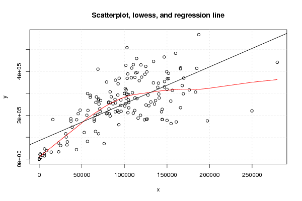
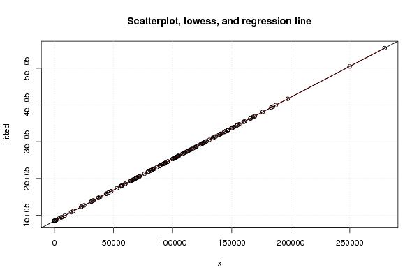
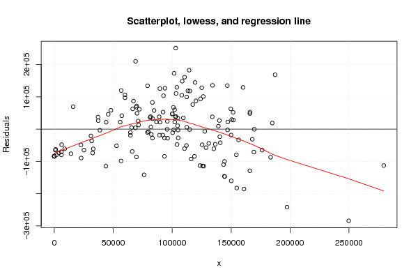
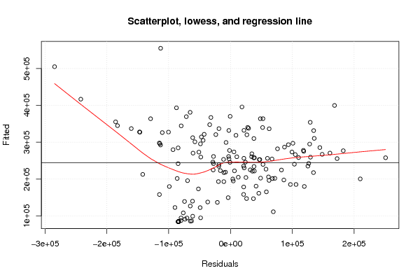
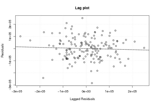
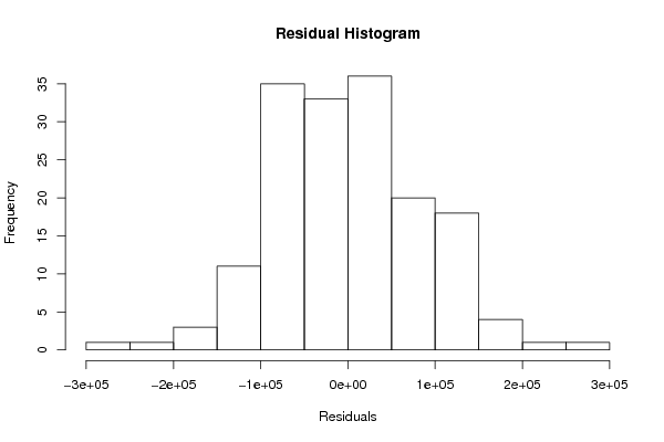
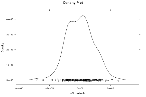
| Title produced by software | Linear Regression Graphical Model Validation | ||||||||||||||||||||||||||||||||||||||||||||||||||||||||||||
| Date of computation | Thu, 22 Dec 2011 15:28:15 -0500 | ||||||||||||||||||||||||||||||||||||||||||||||||||||||||||||
| Cite this page as follows | Statistical Computations at FreeStatistics.org, Office for Research Development and Education, URL https://freestatistics.org/blog/index.php?v=date/2011/Dec/22/t1324585970nph3cz84q2a65c1.htm/, Retrieved Sun, 17 May 2026 11:00:30 +0000 | ||||||||||||||||||||||||||||||||||||||||||||||||||||||||||||
| Statistical Computations at FreeStatistics.org, Office for Research Development and Education, URL https://freestatistics.org/blog/index.php?pk=159953, Retrieved Sun, 17 May 2026 11:00:30 +0000 | |||||||||||||||||||||||||||||||||||||||||||||||||||||||||||||
| QR Codes: | |||||||||||||||||||||||||||||||||||||||||||||||||||||||||||||
|
| |||||||||||||||||||||||||||||||||||||||||||||||||||||||||||||
| Original text written by user: | |||||||||||||||||||||||||||||||||||||||||||||||||||||||||||||
| IsPrivate? | No (this computation is public) | ||||||||||||||||||||||||||||||||||||||||||||||||||||||||||||
| User-defined keywords | |||||||||||||||||||||||||||||||||||||||||||||||||||||||||||||
| Estimated Impact | 391 | ||||||||||||||||||||||||||||||||||||||||||||||||||||||||||||
Tree of Dependent Computations | |||||||||||||||||||||||||||||||||||||||||||||||||||||||||||||
| Family? (F = Feedback message, R = changed R code, M = changed R Module, P = changed Parameters, D = changed Data) | |||||||||||||||||||||||||||||||||||||||||||||||||||||||||||||
| - [Linear Regression Graphical Model Validation] [Colombia Coffee -...] [2008-02-26 10:22:06] [74be16979710d4c4e7c6647856088456] - RM D [Linear Regression Graphical Model Validation] [Regression model 1] [2011-11-15 15:47:03] [74b1e5a3104ff0b2404b2865a63336ad] - PD [Linear Regression Graphical Model Validation] [9-plot] [2011-11-15 20:19:09] [74b1e5a3104ff0b2404b2865a63336ad] - PD [Linear Regression Graphical Model Validation] [Enkelvoudige Line...] [2011-12-22 20:28:15] [f9bdb25068ab2a4592adc645515299ca] [Current] | |||||||||||||||||||||||||||||||||||||||||||||||||||||||||||||
| Feedback Forum | |||||||||||||||||||||||||||||||||||||||||||||||||||||||||||||
Post a new message | |||||||||||||||||||||||||||||||||||||||||||||||||||||||||||||
Dataset | |||||||||||||||||||||||||||||||||||||||||||||||||||||||||||||
| Dataseries X: | |||||||||||||||||||||||||||||||||||||||||||||||||||||||||||||
140824 110459 105079 112098 43929 76173 187326 22807 144408 66485 79089 81625 68788 103297 69446 114948 167949 125081 125818 136588 112431 103037 82317 118906 83515 104581 103129 83243 37110 113344 139165 86652 112302 69652 119442 69867 101629 70168 31081 103925 92622 79011 93487 64520 93473 114360 33032 96125 151911 89256 95676 5950 149695 32551 31701 100087 169707 150491 120192 95893 151715 176225 59900 104767 114799 72128 143592 89626 131072 126817 81351 22618 88977 92059 81897 108146 126372 249771 71154 71571 55918 160141 38692 102812 56622 15986 123534 108535 93879 144551 56750 127654 65594 59938 146975 165904 169265 183500 165986 184923 140358 149959 57224 43750 48029 104978 100046 101047 197426 160902 147172 109432 1168 83248 25162 45724 110529 855 101382 14116 89506 135356 116066 144244 8773 102153 117440 104128 134238 134047 279488 79756 66089 102070 146760 154771 165933 64593 92280 67150 128692 124089 125386 37238 140015 150047 154451 156349 0 6023 0 0 0 0 84601 68946 0 0 1644 6179 3926 52789 0 100350 | |||||||||||||||||||||||||||||||||||||||||||||||||||||||||||||
| Dataseries Y: | |||||||||||||||||||||||||||||||||||||||||||||||||||||||||||||
279055 209884 233939 222117 179751 70849 568125 33186 227332 258874 351915 260484 204003 368577 269455 395936 335567 423110 182016 267365 279428 508849 206722 200004 257139 270815 296850 307100 184160 393860 327660 252512 373013 115602 430118 273950 428077 251349 115658 388812 343783 207021 214344 182398 157164 459455 78800 217932 368086 215843 244765 24188 399093 65029 101097 300488 369627 367127 374193 270099 391871 315924 291391 295075 276201 267432 215924 256641 260919 182961 256967 73566 272362 220707 228835 371391 398210 220401 229333 217623 200046 483074 145943 295224 80953 180759 179344 415550 369093 180679 299505 292260 199481 282361 329281 234577 297995 305984 416463 414359 297080 318283 222281 43287 223456 258249 299566 321797 174736 169579 354041 303273 23668 196743 61857 207339 431443 21054 252805 31961 360401 251240 187003 180842 38214 278173 358276 211775 445926 348017 441946 210700 126320 316128 466139 162279 412099 173802 292443 283913 243609 387072 246963 173260 346748 176654 264767 314070 1 14688 98 455 0 0 284420 410509 0 203 7199 46660 17547 121550 969 242258 | |||||||||||||||||||||||||||||||||||||||||||||||||||||||||||||
Tables (Output of Computation) | |||||||||||||||||||||||||||||||||||||||||||||||||||||||||||||
| |||||||||||||||||||||||||||||||||||||||||||||||||||||||||||||
Figures (Output of Computation) | |||||||||||||||||||||||||||||||||||||||||||||||||||||||||||||
Input Parameters & R Code | |||||||||||||||||||||||||||||||||||||||||||||||||||||||||||||
| Parameters (Session): | |||||||||||||||||||||||||||||||||||||||||||||||||||||||||||||
| par1 = 1 ; par2 = 2 ; par3 = Pearson Chi-Squared ; | |||||||||||||||||||||||||||||||||||||||||||||||||||||||||||||
| Parameters (R input): | |||||||||||||||||||||||||||||||||||||||||||||||||||||||||||||
| par1 = 0 ; | |||||||||||||||||||||||||||||||||||||||||||||||||||||||||||||
| R code (references can be found in the software module): | |||||||||||||||||||||||||||||||||||||||||||||||||||||||||||||
par1 <- as.numeric(par1) | |||||||||||||||||||||||||||||||||||||||||||||||||||||||||||||