Free Statistics
of Irreproducible Research!
Description of Statistical Computation | |||||||||||||||||||||
|---|---|---|---|---|---|---|---|---|---|---|---|---|---|---|---|---|---|---|---|---|---|
| Author's title | |||||||||||||||||||||
| Author | *The author of this computation has been verified* | ||||||||||||||||||||
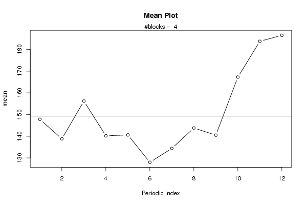
| R Software Module | rwasp_meanplot.wasp | ||||||||||||||||||||
| Title produced by software | Mean Plot | ||||||||||||||||||||
| Date of computation | Tue, 20 Dec 2011 13:10:55 -0500 | ||||||||||||||||||||
| Cite this page as follows | Statistical Computations at FreeStatistics.org, Office for Research Development and Education, URL https://freestatistics.org/blog/index.php?v=date/2011/Dec/20/t1324404770f5cqi8kbahbeycn.htm/, Retrieved Tue, 16 Sep 2025 13:37:29 +0000 | ||||||||||||||||||||
| Statistical Computations at FreeStatistics.org, Office for Research Development and Education, URL https://freestatistics.org/blog/index.php?pk=158113, Retrieved Tue, 16 Sep 2025 13:37:29 +0000 | |||||||||||||||||||||
| QR Codes: | |||||||||||||||||||||
|
| |||||||||||||||||||||
| Original text written by user: | |||||||||||||||||||||
| IsPrivate? | No (this computation is public) | ||||||||||||||||||||
| User-defined keywords | |||||||||||||||||||||
| Estimated Impact | 354 | ||||||||||||||||||||
Tree of Dependent Computations | |||||||||||||||||||||
| Family? (F = Feedback message, R = changed R code, M = changed R Module, P = changed Parameters, D = changed Data) | |||||||||||||||||||||
| - [Bivariate Data Series] [Bivariate dataset] [2008-01-05 23:51:08] [74be16979710d4c4e7c6647856088456] F RMPD [Mean Plot] [Colombia Coffee] [2008-01-07 13:38:24] [74be16979710d4c4e7c6647856088456] - RMPD [Mean Plot] [Mean Plot Car sales] [2010-11-06 16:22:27] [97ad38b1c3b35a5feca8b85f7bc7b3ff] - R D [Mean Plot] [] [2011-11-15 15:57:49] [06c08141d7d783218a8164fd2ea166f2] - D [Mean Plot] [] [2011-12-20 18:10:55] [ce4468323d272130d499477f5e05a6d2] [Current] | |||||||||||||||||||||
| Feedback Forum | |||||||||||||||||||||
Post a new message | |||||||||||||||||||||
Dataset | |||||||||||||||||||||
| Dataseries X: | |||||||||||||||||||||
164 148 152 144 155 125 153 146 138 190 192 192 147 133 163 150 129 131 145 137 138 168 176 188 139 143 150 154 137 129 128 140 143 151 177 184 151 134 164 126 131 125 127 143 143 160 190 182 138 136 152 127 151 130 119 153 | |||||||||||||||||||||
Tables (Output of Computation) | |||||||||||||||||||||
| |||||||||||||||||||||
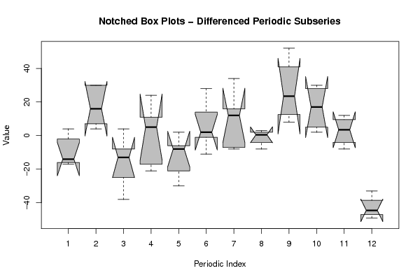
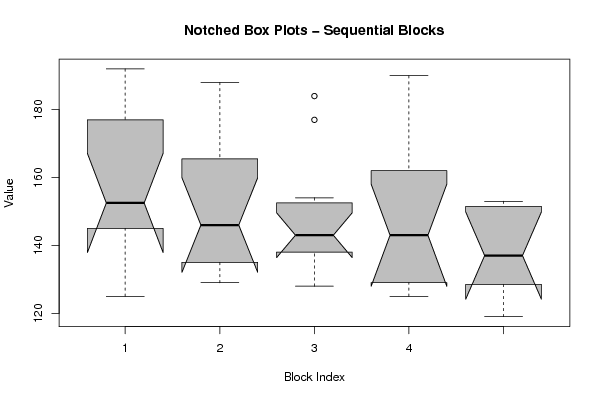
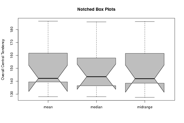
Figures (Output of Computation) | |||||||||||||||||||||
Input Parameters & R Code | |||||||||||||||||||||
| Parameters (Session): | |||||||||||||||||||||
| par1 = 12 ; | |||||||||||||||||||||
| Parameters (R input): | |||||||||||||||||||||
| par1 = 12 ; | |||||||||||||||||||||
| R code (references can be found in the software module): | |||||||||||||||||||||
par1 <- as.numeric(par1) | |||||||||||||||||||||