Free Statistics
of Irreproducible Research!
Description of Statistical Computation | |||||||||||||||||||||||||||||||||||||||||||||||||||||||||||||
|---|---|---|---|---|---|---|---|---|---|---|---|---|---|---|---|---|---|---|---|---|---|---|---|---|---|---|---|---|---|---|---|---|---|---|---|---|---|---|---|---|---|---|---|---|---|---|---|---|---|---|---|---|---|---|---|---|---|---|---|---|---|
| Author's title | |||||||||||||||||||||||||||||||||||||||||||||||||||||||||||||
| Author | *The author of this computation has been verified* | ||||||||||||||||||||||||||||||||||||||||||||||||||||||||||||
| R Software Module | rwasp_linear_regression.wasp | ||||||||||||||||||||||||||||||||||||||||||||||||||||||||||||
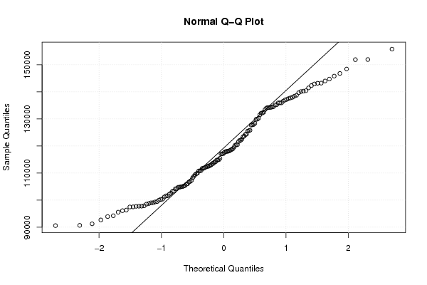
| Title produced by software | Linear Regression Graphical Model Validation | ||||||||||||||||||||||||||||||||||||||||||||||||||||||||||||
| Date of computation | Mon, 19 Dec 2011 10:58:44 -0500 | ||||||||||||||||||||||||||||||||||||||||||||||||||||||||||||
| Cite this page as follows | Statistical Computations at FreeStatistics.org, Office for Research Development and Education, URL https://freestatistics.org/blog/index.php?v=date/2011/Dec/19/t13243103628zulsbe8z43mvqr.htm/, Retrieved Mon, 29 Dec 2025 12:43:42 +0000 | ||||||||||||||||||||||||||||||||||||||||||||||||||||||||||||
| Statistical Computations at FreeStatistics.org, Office for Research Development and Education, URL https://freestatistics.org/blog/index.php?pk=157479, Retrieved Mon, 29 Dec 2025 12:43:42 +0000 | |||||||||||||||||||||||||||||||||||||||||||||||||||||||||||||
| QR Codes: | |||||||||||||||||||||||||||||||||||||||||||||||||||||||||||||
|
| |||||||||||||||||||||||||||||||||||||||||||||||||||||||||||||
| Original text written by user: | |||||||||||||||||||||||||||||||||||||||||||||||||||||||||||||
| IsPrivate? | No (this computation is public) | ||||||||||||||||||||||||||||||||||||||||||||||||||||||||||||
| User-defined keywords | |||||||||||||||||||||||||||||||||||||||||||||||||||||||||||||
| Estimated Impact | 506 | ||||||||||||||||||||||||||||||||||||||||||||||||||||||||||||
Tree of Dependent Computations | |||||||||||||||||||||||||||||||||||||||||||||||||||||||||||||
| Family? (F = Feedback message, R = changed R code, M = changed R Module, P = changed Parameters, D = changed Data) | |||||||||||||||||||||||||||||||||||||||||||||||||||||||||||||
| - [Linear Regression Graphical Model Validation] [Colombia Coffee -...] [2008-02-26 10:22:06] [74be16979710d4c4e7c6647856088456] - RM D [Linear Regression Graphical Model Validation] [Regressiemodel 1] [2010-11-06 16:54:19] [97ad38b1c3b35a5feca8b85f7bc7b3ff] - R P [Linear Regression Graphical Model Validation] [] [2011-11-15 21:43:38] [ec2187f7727da5d5d939740b21b8b68a] - R PD [Linear Regression Graphical Model Validation] [] [2011-12-19 15:58:44] [542c32830549043c4555f1bd78aefedb] [Current] | |||||||||||||||||||||||||||||||||||||||||||||||||||||||||||||
| Feedback Forum | |||||||||||||||||||||||||||||||||||||||||||||||||||||||||||||
Post a new message | |||||||||||||||||||||||||||||||||||||||||||||||||||||||||||||
Dataset | |||||||||||||||||||||||||||||||||||||||||||||||||||||||||||||
| Dataseries X: | |||||||||||||||||||||||||||||||||||||||||||||||||||||||||||||
90604 97527 111940 100280 100009 95558 98533 92694 97920 110933 110855 111716 96348 105425 114874 104199 101166 99010 101607 97492 106088 113536 112475 115491 97733 102591 114783 100397 97772 96128 91261 90686 97792 108848 109989 109453 93945 98750 119043 104776 103262 106735 101600 99358 105240 114079 121637 111747 99496 104992 124255 108258 106940 104939 105896 107287 110783 122139 125823 120480 103296 117121 129924 118589 118062 113597 117161 112893 119657 136562 140446 138744 120324 118113 130257 125510 117986 118316 122075 117573 122566 135934 138394 137999 118780 117907 142932 132200 125666 127958 127718 124368 135241 144734 142320 141481 120471 123422 145829 134572 132156 140265 137771 134035 144016 151905 155791 148440 129862 134264 151952 143191 137242 136993 134431 132523 133486 140120 137521 112193 94256 99047 109761 102160 104792 104341 112430 113034 114197 127876 135199 123663 112578 117104 139703 114961 134222 128390 134197 135963 135936 146803 143231 131510 | |||||||||||||||||||||||||||||||||||||||||||||||||||||||||||||
| Dataseries Y: | |||||||||||||||||||||||||||||||||||||||||||||||||||||||||||||
33145 30912 35591 35832 38376 37971 39824 39908 38969 39553 37387 35119 36446 36041 38790 38281 41972 40483 42092 42255 40476 41254 37280 35192 37077 34265 38876 37447 41159 40153 42528 42681 40643 40724 34054 32587 33955 31396 35638 36474 39387 38233 40619 40340 38856 39325 34675 32695 32975 31210 35283 34247 37126 36582 39230 38672 37886 38118 33627 31880 32016 31900 35825 35818 39208 38581 40367 40033 38946 40144 34764 33328 32890 31171 34811 36879 40339 39112 40765 40730 39298 39653 34418 32387 33363 31463 36570 38031 42459 41764 43278 43024 41588 42396 37942 35454 35860 34110 39102 39584 43408 42247 44096 44083 41815 42668 37079 35454 35963 34673 37967 40127 43416 42659 44164 43134 41827 42188 34683 32762 32441 30076 34246 36224 38787 37849 40351 39865 37832 37867 32681 30910 31321 29857 34472 29353 38552 38344 41196 40955 38706 39368 34145 31123 | |||||||||||||||||||||||||||||||||||||||||||||||||||||||||||||
Tables (Output of Computation) | |||||||||||||||||||||||||||||||||||||||||||||||||||||||||||||
| |||||||||||||||||||||||||||||||||||||||||||||||||||||||||||||
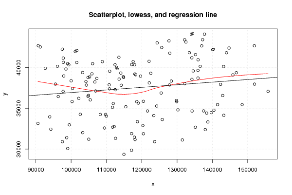
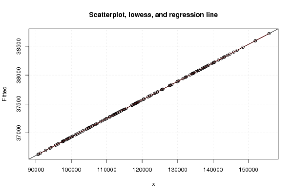
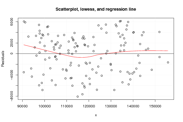
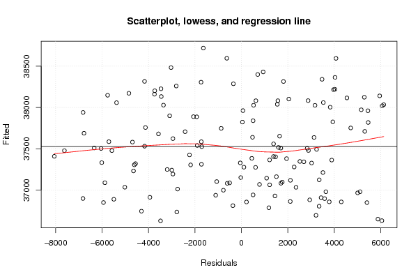
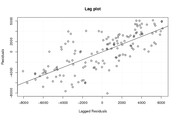
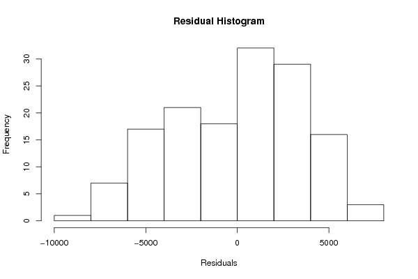
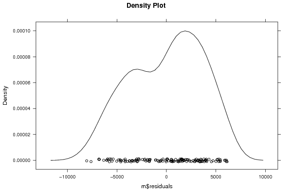
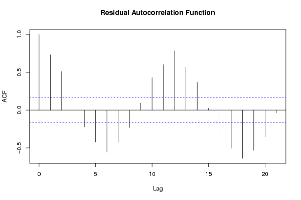
Figures (Output of Computation) | |||||||||||||||||||||||||||||||||||||||||||||||||||||||||||||
Input Parameters & R Code | |||||||||||||||||||||||||||||||||||||||||||||||||||||||||||||
| Parameters (Session): | |||||||||||||||||||||||||||||||||||||||||||||||||||||||||||||
| Parameters (R input): | |||||||||||||||||||||||||||||||||||||||||||||||||||||||||||||
| par1 = 0 ; | |||||||||||||||||||||||||||||||||||||||||||||||||||||||||||||
| R code (references can be found in the software module): | |||||||||||||||||||||||||||||||||||||||||||||||||||||||||||||
par1 <- as.numeric(par1) | |||||||||||||||||||||||||||||||||||||||||||||||||||||||||||||