Repository of Reproducible Computations

Free Statistics

of Irreproducible Research!

Author's title

Author

*The author of this computation has been verified*

R Software Module

rwasp_pairs.wasp

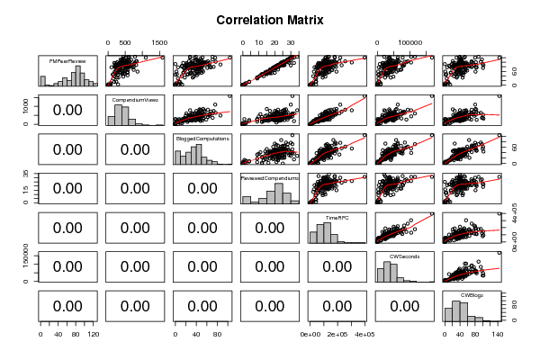
Title produced by software

Kendall tau Correlation Matrix

Date of computation

Thu, 15 Dec 2011 11:14:06 -0500

Cite this page as follows

Statistical Computations at FreeStatistics.org, Office for Research Development and Education, URL https://freestatistics.org/blog/index.php?v=date/2011/Dec/15/t1323965694wddvoxja1t4qkyr.htm/, Retrieved Mon, 29 Apr 2024 06:54:54 +0000

Statistical Computations at FreeStatistics.org, Office for Research Development and Education, URL https://freestatistics.org/blog/index.php?pk=155543, Retrieved Mon, 29 Apr 2024 06:54:54 +0000

QR Codes:

Paste this QR Code to cite your computation.

Original text written by user:

IsPrivate?

No (this computation is public)

User-defined keywords

Estimated Impact

Family? (F = Feedback message, R = changed R code, M = changed R Module, P = changed Parameters, D = changed Data)

-     [Kendall tau Correlation Matrix] [] [2010-12-05 17:44:33] [b98453cac15ba1066b407e146608df68]
- RMPD  [Kendall tau Correlation Matrix] [Pearson Corr Matrix] [2011-12-15 16:11:32] [15a5dd358825f04074b70fc847ec6454]
-   P       [Kendall tau Correlation Matrix] [Kendall Tau Corr ...] [2011-12-15 16:14:06] [614dd89c388120cee0dd25886939832b] [Current]
- R  D        [Kendall tau Correlation Matrix] [PAPER] [2011-12-17 14:27:02] [27e29806e0b1d1351a97bc4ee4116294] 

Feedback Forum

Post a new message

Dataseries X:

Download CSV

Histogram

Boxplots

70	500	20	18	129404	22622	28
68	329	38	17	130358	73570	39
0	72	0	0	7215	1929	0
68	584	49	22	112861	36294	54
120	1100	76	30	219904	62378	80
120	1585	104	31	397355	167760	144
72	442	37	19	117604	52443	36
96	321	53	25	126737	57283	48
109	406	42	30	99729	36614	42
104	818	62	26	256310	93268	71
54	568	50	20	113066	35439	49
98	556	65	25	157228	72405	74
49	494	28	15	69952	24044	27
88	818	48	22	152673	55909	83
57	338	42	16	130642	44689	31
74	419	47	19	125769	49319	28
112	364	71	28	123467	62075	98
45	284	0	12	56232	2341	2
110	674	50	28	108330	40551	43
39	188	12	13	22762	11621	24
55	286	16	14	48554	18741	16
102	640	77	27	182081	84202	95
96	520	29	25	140857	15334	22
86	532	38	30	93773	28024	33
78	547	50	21	133398	53306	45
64	428	33	17	113933	37918	59
82	561	49	22	153851	54819	66
100	266	59	28	140711	89058	70
99	783	55	26	303804	103354	56
67	746	40	17	161651	70239	55
87	394	40	23	123344	33045	27
65	482	51	20	157640	63852	37
43	568	41	11	91279	30905	48
80	746	73	20	189374	24242	26
84	668	51	21	178768	78907	64
0	0	0	0	0	0	0
105	835	46	27	175403	36005	21
51	464	44	14	92342	31972	44
98	418	31	29	100023	35853	36
124	607	71	31	178277	115301	89
75	539	61	19	145062	47689	101
120	519	28	30	110980	34223	31
84	309	21	23	86039	43431	65
82	647	42	21	125481	52220	71
87	321	44	22	95535	33863	102
78	261	40	21	126456	46879	53
97	180	15	32	61554	23228	41
76	576	46	19	164752	42827	46
104	544	43	26	159121	65765	37
93	758	47	25	129362	38167	51
82	205	12	22	48188	14812	14
73	317	46	19	95461	32615	40
87	709	56	24	229864	82188	77
95	590	47	26	191094	51763	51
105	526	48	27	150640	59325	43
37	443	35	10	111388	48976	33
96	419	44	26	165098	43384	47
88	205	25	23	63205	26692	31
83	310	47	21	109102	53279	31
124	785	28	34	137303	20652	40
116	434	48	29	125304	38338	42
76	576	32	19	85332	36735	35
65	317	28	19	95808	42764	40
86	288	31	23	83419	44331	30
85	285	13	22	101723	41354	11
107	391	38	29	94982	47879	41
124	446	39	31	129700	103793	53
78	715	68	21	113325	52235	82
83	208	32	21	81518	49825	41
78	101	5	21	31970	4105	6
59	858	53	15	192268	58687	81
33	302	33	9	91086	40745	47
92	360	54	23	80820	33187	100
52	411	36	18	83261	14063	46
121	561	52	31	116290	37407	38
92	292	0	25	56544	7190	0
99	492	52	24	116173	49562	45
86	669	45	22	111488	76324	56
75	253	16	21	60138	21928	18
96	366	33	26	73422	27860	54
81	192	48	22	67751	28078	37
104	616	33	26	213351	49577	40
76	221	24	20	51185	28145	37
90	438	37	25	97181	36241	36
75	247	17	19	45100	10824	34
86	388	32	22	115801	46892	49
100	541	55	25	186310	61264	82
88	233	39	22	71960	22933	36
80	333	31	21	80105	20787	33
73	422	26	20	103613	43978	55
88	452	37	23	98707	51305	50
79	584	66	22	136234	55593	71
81	366	35	21	136781	51648	31
48	406	24	12	105863	30552	42
33	254	18	9	38775	23470	31
120	606	37	32	179997	77530	51
90	491	86	24	169406	57299	64
2	67	13	1	19349	9604	14
96	607	21	24	153069	34684	37
86	597	32	25	109510	41094	37
15	240	8	4	43803	3439	8
48	219	38	15	47062	25171	38
81	349	45	21	110845	23437	23
84	241	24	23	92517	34086	22
46	136	23	12	58660	24649	18
59	194	2	16	27676	2342	1
96	222	52	24	98550	45571	48
29	153	5	9	43646	3255	5
0	0	0	0	0	0	0
83	251	43	23	67312	30002	46
63	240	18	17	57359	19360	33
68	358	44	18	104330	43320	41
84	302	45	21	70369	35513	57
54	267	29	17	65494	23536	49
0	14	0	0	3616	0	0
0	0	0	0	0	0	0
75	287	32	20	143931	54438	45
87	476	65	26	117946	56812	78
104	509	26	26	131175	33838	46
80	243	24	20	84336	32366	25
3	292	7	1	43410	13	1
93	410	62	24	136250	55082	59
55	217	30	14	79015	31334	29
96	422	49	26	92937	16612	26
48	160	3	12	57586	5084	4
8	75	10	2	19764	9927	10
60	412	42	16	105757	47413	43
84	309	18	22	97213	27389	36
112	417	40	28	113402	30425	41
8	79	1	2	11796	0	0
0	25	0	0	7627	0	0
52	431	29	17	121085	33510	32
4	11	0	1	6836	0	0
57	564	46	17	139563	40389	53
0	6	5	0	5118	0	0
14	183	8	4	40248	6012	6
0	0	0	0	0	0	0
91	295	21	25	95079	22205	18
89	230	21	26	80763	17231	26
0	27	0	0	7131	0	0
0	14	0	0	4194	0	0
54	240	15	15	60378	11017	16
77	251	47	20	109173	46741	84
76	347	17	19	83484	39869	22

Summary of computational transaction
Raw Input	view raw input (R code)
Raw Output	view raw output of R engine
Computing time	1 seconds
R Server	'Herman Ole Andreas Wold' @ wold.wessa.net

\begin{tabular}{lllllllll}
\hline
Summary of computational transaction \tabularnewline
Raw Input & view raw input (R code)  \tabularnewline
Raw Output & view raw output of R engine  \tabularnewline
Computing time & 1 seconds \tabularnewline
R Server & 'Herman Ole Andreas Wold' @ wold.wessa.net \tabularnewline
\hline
\end{tabular}
%Source: https://freestatistics.org/blog/index.php?pk=155543&T=0

[TABLE]
[ROW][C]Summary of computational transaction[/C][/ROW]
[ROW][C]Raw Input[/C][C]view raw input (R code) [/C][/ROW]
[ROW][C]Raw Output[/C][C]view raw output of R engine [/C][/ROW]
[ROW][C]Computing time[/C][C]1 seconds[/C][/ROW]
[ROW][C]R Server[/C][C]'Herman Ole Andreas Wold' @ wold.wessa.net[/C][/ROW]
[/TABLE]
Source: https://freestatistics.org/blog/index.php?pk=155543&T=0

Globally Unique Identifier (entire table): ba.freestatistics.org/blog/index.php?pk=155543&T=0

As an alternative you can also use a QR Code:

The GUIDs for individual cells are displayed in the table below:

Summary of computational transaction
Raw Input	view raw input (R code)
Raw Output	view raw output of R engine
Computing time	1 seconds
R Server	'Herman Ole Andreas Wold' @ wold.wessa.net

Correlations for all pairs of data series (method=kendall)
	FMPeerReview	CompendiumViews	BloggedComputations	ReviewedCompendiums	TimeRFC	CWSeconds	CWBlogs
FMPeerReview	1	0.405	0.416	0.902	0.459	0.418	0.37
CompendiumViews	0.405	1	0.534	0.403	0.673	0.515	0.483
BloggedComputations	0.416	0.534	1	0.41	0.596	0.62	0.645
ReviewedCompendiums	0.902	0.403	0.41	1	0.436	0.4	0.368
TimeRFC	0.459	0.673	0.596	0.436	1	0.67	0.512
CWSeconds	0.418	0.515	0.62	0.4	0.67	1	0.615
CWBlogs	0.37	0.483	0.645	0.368	0.512	0.615	1

\begin{tabular}{lllllllll}
\hline
Correlations for all pairs of data series (method=kendall) \tabularnewline
  & FMPeerReview & CompendiumViews & BloggedComputations & ReviewedCompendiums & TimeRFC & CWSeconds & CWBlogs \tabularnewline
FMPeerReview & 1 & 0.405 & 0.416 & 0.902 & 0.459 & 0.418 & 0.37 \tabularnewline
CompendiumViews & 0.405 & 1 & 0.534 & 0.403 & 0.673 & 0.515 & 0.483 \tabularnewline
BloggedComputations & 0.416 & 0.534 & 1 & 0.41 & 0.596 & 0.62 & 0.645 \tabularnewline
ReviewedCompendiums & 0.902 & 0.403 & 0.41 & 1 & 0.436 & 0.4 & 0.368 \tabularnewline
TimeRFC & 0.459 & 0.673 & 0.596 & 0.436 & 1 & 0.67 & 0.512 \tabularnewline
CWSeconds & 0.418 & 0.515 & 0.62 & 0.4 & 0.67 & 1 & 0.615 \tabularnewline
CWBlogs & 0.37 & 0.483 & 0.645 & 0.368 & 0.512 & 0.615 & 1 \tabularnewline
\hline
\end{tabular}
%Source: https://freestatistics.org/blog/index.php?pk=155543&T=1

[TABLE]
[ROW][C]Correlations for all pairs of data series (method=kendall)[/C][/ROW]
[ROW][C] [/C][C]FMPeerReview[/C][C]CompendiumViews[/C][C]BloggedComputations[/C][C]ReviewedCompendiums[/C][C]TimeRFC[/C][C]CWSeconds[/C][C]CWBlogs[/C][/ROW]
[ROW][C]FMPeerReview[/C][C]1[/C][C]0.405[/C][C]0.416[/C][C]0.902[/C][C]0.459[/C][C]0.418[/C][C]0.37[/C][/ROW]
[ROW][C]CompendiumViews[/C][C]0.405[/C][C]1[/C][C]0.534[/C][C]0.403[/C][C]0.673[/C][C]0.515[/C][C]0.483[/C][/ROW]
[ROW][C]BloggedComputations[/C][C]0.416[/C][C]0.534[/C][C]1[/C][C]0.41[/C][C]0.596[/C][C]0.62[/C][C]0.645[/C][/ROW]
[ROW][C]ReviewedCompendiums[/C][C]0.902[/C][C]0.403[/C][C]0.41[/C][C]1[/C][C]0.436[/C][C]0.4[/C][C]0.368[/C][/ROW]
[ROW][C]TimeRFC[/C][C]0.459[/C][C]0.673[/C][C]0.596[/C][C]0.436[/C][C]1[/C][C]0.67[/C][C]0.512[/C][/ROW]
[ROW][C]CWSeconds[/C][C]0.418[/C][C]0.515[/C][C]0.62[/C][C]0.4[/C][C]0.67[/C][C]1[/C][C]0.615[/C][/ROW]
[ROW][C]CWBlogs[/C][C]0.37[/C][C]0.483[/C][C]0.645[/C][C]0.368[/C][C]0.512[/C][C]0.615[/C][C]1[/C][/ROW]
[/TABLE]
Source: https://freestatistics.org/blog/index.php?pk=155543&T=1

Globally Unique Identifier (entire table): ba.freestatistics.org/blog/index.php?pk=155543&T=1

As an alternative you can also use a QR Code:

The GUIDs for individual cells are displayed in the table below:

Correlations for all pairs of data series (method=kendall)
	FMPeerReview	CompendiumViews	BloggedComputations	ReviewedCompendiums	TimeRFC	CWSeconds	CWBlogs
FMPeerReview	1	0.405	0.416	0.902	0.459	0.418	0.37
CompendiumViews	0.405	1	0.534	0.403	0.673	0.515	0.483
BloggedComputations	0.416	0.534	1	0.41	0.596	0.62	0.645
ReviewedCompendiums	0.902	0.403	0.41	1	0.436	0.4	0.368
TimeRFC	0.459	0.673	0.596	0.436	1	0.67	0.512
CWSeconds	0.418	0.515	0.62	0.4	0.67	1	0.615
CWBlogs	0.37	0.483	0.645	0.368	0.512	0.615	1

Correlations for all pairs of data series with p-values
pair	Pearson r	Spearman rho	Kendall tau
FMPeerReview;CompendiumViews	0.6194	0.5528	0.4045
p-value	(0)	(0)	(0)
FMPeerReview;BloggedComputations	0.6569	0.5672	0.4161
p-value	(0)	(0)	(0)
FMPeerReview;ReviewedCompendiums	0.9843	0.9757	0.9023
p-value	(0)	(0)	(0)
FMPeerReview;TimeRFC	0.6762	0.6214	0.4594
p-value	(0)	(0)	(0)
FMPeerReview;CWSeconds	0.6319	0.5658	0.4176
p-value	(0)	(0)	(0)
FMPeerReview;CWBlogs	0.5964	0.5151	0.3701
p-value	(0)	(0)	(0)
CompendiumViews;BloggedComputations	0.7426	0.7087	0.5338
p-value	(0)	(0)	(0)
CompendiumViews;ReviewedCompendiums	0.6072	0.5418	0.4026
p-value	(0)	(0)	(0)
CompendiumViews;TimeRFC	0.8774	0.8477	0.6734
p-value	(0)	(0)	(0)
CompendiumViews;CWSeconds	0.7185	0.6858	0.5149
p-value	(0)	(0)	(0)
CompendiumViews;CWBlogs	0.6801	0.6491	0.4831
p-value	(0)	(0)	(0)
BloggedComputations;ReviewedCompendiums	0.6442	0.5498	0.4102
p-value	(0)	(0)	(0)
BloggedComputations;TimeRFC	0.7935	0.7726	0.5963
p-value	(0)	(0)	(0)
BloggedComputations;CWSeconds	0.7909	0.7855	0.6202
p-value	(0)	(0)	(0)
BloggedComputations;CWBlogs	0.8392	0.7989	0.6452
p-value	(0)	(0)	(0)
ReviewedCompendiums;TimeRFC	0.6525	0.5897	0.4364
p-value	(0)	(0)	(0)
ReviewedCompendiums;CWSeconds	0.6038	0.5335	0.3997
p-value	(0)	(0)	(0)
ReviewedCompendiums;CWBlogs	0.5844	0.5041	0.3677
p-value	(0)	(0)	(0)
TimeRFC;CWSeconds	0.854	0.8345	0.6697
p-value	(0)	(0)	(0)
TimeRFC;CWBlogs	0.7105	0.6834	0.5121
p-value	(0)	(0)	(0)
CWSeconds;CWBlogs	0.7797	0.7843	0.6153
p-value	(0)	(0)	(0)

\begin{tabular}{lllllllll}
\hline
Correlations for all pairs of data series with p-values \tabularnewline
pair & Pearson r & Spearman rho & Kendall tau \tabularnewline
FMPeerReview;CompendiumViews & 0.6194 & 0.5528 & 0.4045 \tabularnewline
p-value & (0) & (0) & (0) \tabularnewline
FMPeerReview;BloggedComputations & 0.6569 & 0.5672 & 0.4161 \tabularnewline
p-value & (0) & (0) & (0) \tabularnewline
FMPeerReview;ReviewedCompendiums & 0.9843 & 0.9757 & 0.9023 \tabularnewline
p-value & (0) & (0) & (0) \tabularnewline
FMPeerReview;TimeRFC & 0.6762 & 0.6214 & 0.4594 \tabularnewline
p-value & (0) & (0) & (0) \tabularnewline
FMPeerReview;CWSeconds & 0.6319 & 0.5658 & 0.4176 \tabularnewline
p-value & (0) & (0) & (0) \tabularnewline
FMPeerReview;CWBlogs & 0.5964 & 0.5151 & 0.3701 \tabularnewline
p-value & (0) & (0) & (0) \tabularnewline
CompendiumViews;BloggedComputations & 0.7426 & 0.7087 & 0.5338 \tabularnewline
p-value & (0) & (0) & (0) \tabularnewline
CompendiumViews;ReviewedCompendiums & 0.6072 & 0.5418 & 0.4026 \tabularnewline
p-value & (0) & (0) & (0) \tabularnewline
CompendiumViews;TimeRFC & 0.8774 & 0.8477 & 0.6734 \tabularnewline
p-value & (0) & (0) & (0) \tabularnewline
CompendiumViews;CWSeconds & 0.7185 & 0.6858 & 0.5149 \tabularnewline
p-value & (0) & (0) & (0) \tabularnewline
CompendiumViews;CWBlogs & 0.6801 & 0.6491 & 0.4831 \tabularnewline
p-value & (0) & (0) & (0) \tabularnewline
BloggedComputations;ReviewedCompendiums & 0.6442 & 0.5498 & 0.4102 \tabularnewline
p-value & (0) & (0) & (0) \tabularnewline
BloggedComputations;TimeRFC & 0.7935 & 0.7726 & 0.5963 \tabularnewline
p-value & (0) & (0) & (0) \tabularnewline
BloggedComputations;CWSeconds & 0.7909 & 0.7855 & 0.6202 \tabularnewline
p-value & (0) & (0) & (0) \tabularnewline
BloggedComputations;CWBlogs & 0.8392 & 0.7989 & 0.6452 \tabularnewline
p-value & (0) & (0) & (0) \tabularnewline
ReviewedCompendiums;TimeRFC & 0.6525 & 0.5897 & 0.4364 \tabularnewline
p-value & (0) & (0) & (0) \tabularnewline
ReviewedCompendiums;CWSeconds & 0.6038 & 0.5335 & 0.3997 \tabularnewline
p-value & (0) & (0) & (0) \tabularnewline
ReviewedCompendiums;CWBlogs & 0.5844 & 0.5041 & 0.3677 \tabularnewline
p-value & (0) & (0) & (0) \tabularnewline
TimeRFC;CWSeconds & 0.854 & 0.8345 & 0.6697 \tabularnewline
p-value & (0) & (0) & (0) \tabularnewline
TimeRFC;CWBlogs & 0.7105 & 0.6834 & 0.5121 \tabularnewline
p-value & (0) & (0) & (0) \tabularnewline
CWSeconds;CWBlogs & 0.7797 & 0.7843 & 0.6153 \tabularnewline
p-value & (0) & (0) & (0) \tabularnewline
\hline
\end{tabular}
%Source: https://freestatistics.org/blog/index.php?pk=155543&T=2

[TABLE]
[ROW][C]Correlations for all pairs of data series with p-values[/C][/ROW]
[ROW][C]pair[/C][C]Pearson r[/C][C]Spearman rho[/C][C]Kendall tau[/C][/ROW]
[ROW][C]FMPeerReview;CompendiumViews[/C][C]0.6194[/C][C]0.5528[/C][C]0.4045[/C][/ROW]
[ROW][C]p-value[/C][C](0)[/C][C](0)[/C][C](0)[/C][/ROW]
[ROW][C]FMPeerReview;BloggedComputations[/C][C]0.6569[/C][C]0.5672[/C][C]0.4161[/C][/ROW]
[ROW][C]p-value[/C][C](0)[/C][C](0)[/C][C](0)[/C][/ROW]
[ROW][C]FMPeerReview;ReviewedCompendiums[/C][C]0.9843[/C][C]0.9757[/C][C]0.9023[/C][/ROW]
[ROW][C]p-value[/C][C](0)[/C][C](0)[/C][C](0)[/C][/ROW]
[ROW][C]FMPeerReview;TimeRFC[/C][C]0.6762[/C][C]0.6214[/C][C]0.4594[/C][/ROW]
[ROW][C]p-value[/C][C](0)[/C][C](0)[/C][C](0)[/C][/ROW]
[ROW][C]FMPeerReview;CWSeconds[/C][C]0.6319[/C][C]0.5658[/C][C]0.4176[/C][/ROW]
[ROW][C]p-value[/C][C](0)[/C][C](0)[/C][C](0)[/C][/ROW]
[ROW][C]FMPeerReview;CWBlogs[/C][C]0.5964[/C][C]0.5151[/C][C]0.3701[/C][/ROW]
[ROW][C]p-value[/C][C](0)[/C][C](0)[/C][C](0)[/C][/ROW]
[ROW][C]CompendiumViews;BloggedComputations[/C][C]0.7426[/C][C]0.7087[/C][C]0.5338[/C][/ROW]
[ROW][C]p-value[/C][C](0)[/C][C](0)[/C][C](0)[/C][/ROW]
[ROW][C]CompendiumViews;ReviewedCompendiums[/C][C]0.6072[/C][C]0.5418[/C][C]0.4026[/C][/ROW]
[ROW][C]p-value[/C][C](0)[/C][C](0)[/C][C](0)[/C][/ROW]
[ROW][C]CompendiumViews;TimeRFC[/C][C]0.8774[/C][C]0.8477[/C][C]0.6734[/C][/ROW]
[ROW][C]p-value[/C][C](0)[/C][C](0)[/C][C](0)[/C][/ROW]
[ROW][C]CompendiumViews;CWSeconds[/C][C]0.7185[/C][C]0.6858[/C][C]0.5149[/C][/ROW]
[ROW][C]p-value[/C][C](0)[/C][C](0)[/C][C](0)[/C][/ROW]
[ROW][C]CompendiumViews;CWBlogs[/C][C]0.6801[/C][C]0.6491[/C][C]0.4831[/C][/ROW]
[ROW][C]p-value[/C][C](0)[/C][C](0)[/C][C](0)[/C][/ROW]
[ROW][C]BloggedComputations;ReviewedCompendiums[/C][C]0.6442[/C][C]0.5498[/C][C]0.4102[/C][/ROW]
[ROW][C]p-value[/C][C](0)[/C][C](0)[/C][C](0)[/C][/ROW]
[ROW][C]BloggedComputations;TimeRFC[/C][C]0.7935[/C][C]0.7726[/C][C]0.5963[/C][/ROW]
[ROW][C]p-value[/C][C](0)[/C][C](0)[/C][C](0)[/C][/ROW]
[ROW][C]BloggedComputations;CWSeconds[/C][C]0.7909[/C][C]0.7855[/C][C]0.6202[/C][/ROW]
[ROW][C]p-value[/C][C](0)[/C][C](0)[/C][C](0)[/C][/ROW]
[ROW][C]BloggedComputations;CWBlogs[/C][C]0.8392[/C][C]0.7989[/C][C]0.6452[/C][/ROW]
[ROW][C]p-value[/C][C](0)[/C][C](0)[/C][C](0)[/C][/ROW]
[ROW][C]ReviewedCompendiums;TimeRFC[/C][C]0.6525[/C][C]0.5897[/C][C]0.4364[/C][/ROW]
[ROW][C]p-value[/C][C](0)[/C][C](0)[/C][C](0)[/C][/ROW]
[ROW][C]ReviewedCompendiums;CWSeconds[/C][C]0.6038[/C][C]0.5335[/C][C]0.3997[/C][/ROW]
[ROW][C]p-value[/C][C](0)[/C][C](0)[/C][C](0)[/C][/ROW]
[ROW][C]ReviewedCompendiums;CWBlogs[/C][C]0.5844[/C][C]0.5041[/C][C]0.3677[/C][/ROW]
[ROW][C]p-value[/C][C](0)[/C][C](0)[/C][C](0)[/C][/ROW]
[ROW][C]TimeRFC;CWSeconds[/C][C]0.854[/C][C]0.8345[/C][C]0.6697[/C][/ROW]
[ROW][C]p-value[/C][C](0)[/C][C](0)[/C][C](0)[/C][/ROW]
[ROW][C]TimeRFC;CWBlogs[/C][C]0.7105[/C][C]0.6834[/C][C]0.5121[/C][/ROW]
[ROW][C]p-value[/C][C](0)[/C][C](0)[/C][C](0)[/C][/ROW]
[ROW][C]CWSeconds;CWBlogs[/C][C]0.7797[/C][C]0.7843[/C][C]0.6153[/C][/ROW]
[ROW][C]p-value[/C][C](0)[/C][C](0)[/C][C](0)[/C][/ROW]
[/TABLE]
Source: https://freestatistics.org/blog/index.php?pk=155543&T=2

Globally Unique Identifier (entire table): ba.freestatistics.org/blog/index.php?pk=155543&T=2

As an alternative you can also use a QR Code:

The GUIDs for individual cells are displayed in the table below:

Correlations for all pairs of data series with p-values
pair	Pearson r	Spearman rho	Kendall tau
FMPeerReview;CompendiumViews	0.6194	0.5528	0.4045
p-value	(0)	(0)	(0)
FMPeerReview;BloggedComputations	0.6569	0.5672	0.4161
p-value	(0)	(0)	(0)
FMPeerReview;ReviewedCompendiums	0.9843	0.9757	0.9023
p-value	(0)	(0)	(0)
FMPeerReview;TimeRFC	0.6762	0.6214	0.4594
p-value	(0)	(0)	(0)
FMPeerReview;CWSeconds	0.6319	0.5658	0.4176
p-value	(0)	(0)	(0)
FMPeerReview;CWBlogs	0.5964	0.5151	0.3701
p-value	(0)	(0)	(0)
CompendiumViews;BloggedComputations	0.7426	0.7087	0.5338
p-value	(0)	(0)	(0)
CompendiumViews;ReviewedCompendiums	0.6072	0.5418	0.4026
p-value	(0)	(0)	(0)
CompendiumViews;TimeRFC	0.8774	0.8477	0.6734
p-value	(0)	(0)	(0)
CompendiumViews;CWSeconds	0.7185	0.6858	0.5149
p-value	(0)	(0)	(0)
CompendiumViews;CWBlogs	0.6801	0.6491	0.4831
p-value	(0)	(0)	(0)
BloggedComputations;ReviewedCompendiums	0.6442	0.5498	0.4102
p-value	(0)	(0)	(0)
BloggedComputations;TimeRFC	0.7935	0.7726	0.5963
p-value	(0)	(0)	(0)
BloggedComputations;CWSeconds	0.7909	0.7855	0.6202
p-value	(0)	(0)	(0)
BloggedComputations;CWBlogs	0.8392	0.7989	0.6452
p-value	(0)	(0)	(0)
ReviewedCompendiums;TimeRFC	0.6525	0.5897	0.4364
p-value	(0)	(0)	(0)
ReviewedCompendiums;CWSeconds	0.6038	0.5335	0.3997
p-value	(0)	(0)	(0)
ReviewedCompendiums;CWBlogs	0.5844	0.5041	0.3677
p-value	(0)	(0)	(0)
TimeRFC;CWSeconds	0.854	0.8345	0.6697
p-value	(0)	(0)	(0)
TimeRFC;CWBlogs	0.7105	0.6834	0.5121
p-value	(0)	(0)	(0)
CWSeconds;CWBlogs	0.7797	0.7843	0.6153
p-value	(0)	(0)	(0)

Figure 1

PNG link

Postscript link

PDF link

Parameters (Session):

par1 = kendall ;

Parameters (R input):

par1 = kendall ;

R code (references can be found in the software module):

panel.tau <- function(x, y, digits=2, prefix='', cex.cor)
{
usr <- par('usr'); on.exit(par(usr))
par(usr = c(0, 1, 0, 1))
rr <- cor.test(x, y, method=par1)
r <- round(rr$p.value,2)
txt <- format(c(r, 0.123456789), digits=digits)[1]
txt <- paste(prefix, txt, sep='')
if(missing(cex.cor)) cex <- 0.5/strwidth(txt)
text(0.5, 0.5, txt, cex = cex)
}
panel.hist <- function(x, ...)
{
usr <- par('usr'); on.exit(par(usr))
par(usr = c(usr[1:2], 0, 1.5) )
h <- hist(x, plot = FALSE)
breaks <- h$breaks; nB <- length(breaks)
y <- h$counts; y <- y/max(y)
rect(breaks[-nB], 0, breaks[-1], y, col='grey', ...)
}
bitmap(file='test1.png')
pairs(t(y),diag.panel=panel.hist, upper.panel=panel.smooth, lower.panel=panel.tau, main=main)
dev.off()
load(file='createtable')
n <- length(y[,1])
n
a<-table.start()
a<-table.row.start(a)
a<-table.element(a,paste('Correlations for all pairs of data series (method=',par1,')',sep=''),n+1,TRUE)
a<-table.row.end(a)
a<-table.row.start(a)
a<-table.element(a,' ',header=TRUE)
for (i in 1:n) {
a<-table.element(a,dimnames(t(x))[[2]][i],header=TRUE)
}
a<-table.row.end(a)
for (i in 1:n) {
a<-table.row.start(a)
a<-table.element(a,dimnames(t(x))[[2]][i],header=TRUE)
for (j in 1:n) {
r <- cor.test(y[i,],y[j,],method=par1)
a<-table.element(a,round(r$estimate,3))
}
a<-table.row.end(a)
}
a<-table.end(a)
table.save(a,file='mytable.tab')
a<-table.start()
a<-table.row.start(a)
a<-table.element(a,'Correlations for all pairs of data series with p-values',4,TRUE)
a<-table.row.end(a)
a<-table.row.start(a)
a<-table.element(a,'pair',1,TRUE)
a<-table.element(a,'Pearson r',1,TRUE)
a<-table.element(a,'Spearman rho',1,TRUE)
a<-table.element(a,'Kendall tau',1,TRUE)
a<-table.row.end(a)
cor.test(y[1,],y[2,],method=par1)
for (i in 1:(n-1))
{
for (j in (i+1):n)
{
a<-table.row.start(a)
dum <- paste(dimnames(t(x))[[2]][i],';',dimnames(t(x))[[2]][j],sep='')
a<-table.element(a,dum,header=TRUE)
rp <- cor.test(y[i,],y[j,],method='pearson')
a<-table.element(a,round(rp$estimate,4))
rs <- cor.test(y[i,],y[j,],method='spearman')
a<-table.element(a,round(rs$estimate,4))
rk <- cor.test(y[i,],y[j,],method='kendall')
a<-table.element(a,round(rk$estimate,4))
a<-table.row.end(a)
a<-table.row.start(a)
a<-table.element(a,'p-value',header=T)
a<-table.element(a,paste('(',round(rp$p.value,4),')',sep=''))
a<-table.element(a,paste('(',round(rs$p.value,4),')',sep=''))
a<-table.element(a,paste('(',round(rk$p.value,4),')',sep=''))
a<-table.row.end(a)
}
}
a<-table.end(a)
table.save(a,file='mytable1.tab')

Free Statistics

Description of Statistical Computation

Tree of Dependent Computations

Dataset

Tables (Output of Computation)

Figures (Output of Computation)

Input Parameters & R Code