Repository of Reproducible Computations

Free Statistics

of Irreproducible Research!

Author's title

Author

*Unverified author*

R Software Module

rwasp_autocorrelation.wasp

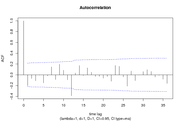
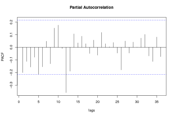
Title produced by software

(Partial) Autocorrelation Function

Date of computation

Sat, 10 Dec 2011 07:56:10 -0500

Cite this page as follows

Statistical Computations at FreeStatistics.org, Office for Research Development and Education, URL https://freestatistics.org/blog/index.php?v=date/2011/Dec/10/t13235218033tj05csb7ne9n5d.htm/, Retrieved Mon, 29 Apr 2024 04:01:46 +0000

Statistical Computations at FreeStatistics.org, Office for Research Development and Education, URL https://freestatistics.org/blog/index.php?pk=153504, Retrieved Mon, 29 Apr 2024 04:01:46 +0000

QR Codes:

Paste this QR Code to cite your computation.

Original text written by user:

IsPrivate?

No (this computation is public)

User-defined keywords

Estimated Impact

136

Family? (F = Feedback message, R = changed R code, M = changed R Module, P = changed Parameters, D = changed Data)

-     [Univariate Explorative Data Analysis] [Run Sequence gebo...] [2008-12-12 13:32:37] [76963dc1903f0f612b6153510a3818cf]
- R  D  [Univariate Explorative Data Analysis] [Run Sequence gebo...] [2008-12-17 12:14:40] [76963dc1903f0f612b6153510a3818cf]
-         [Univariate Explorative Data Analysis] [Run Sequence Plot...] [2008-12-22 18:19:51] [1ce0d16c8f4225c977b42c8fa93bc163]
- RMP       [(Partial) Autocorrelation Function] [Identifying Integ...] [2009-11-22 12:16:10] [b98453cac15ba1066b407e146608df68]
-   PD        [(Partial) Autocorrelation Function] [ws8_2] [2009-11-24 20:22:15] [8b1aef4e7013bd33fbc2a5833375c5f5]
-   P           [(Partial) Autocorrelation Function] [WS8_seizonaliteit1] [2009-11-25 17:44:58] [8b1aef4e7013bd33fbc2a5833375c5f5]
-    D            [(Partial) Autocorrelation Function] [paper timeserie A...] [2010-12-06 20:13:10] [814f53995537cd15c528d8efbf1cf544]
- R  D                [(Partial) Autocorrelation Function] [] [2011-12-10 12:56:10] [d41d8cd98f00b204e9800998ecf8427e] [Current]
-   PD                  [(Partial) Autocorrelation Function] [] [2011-12-10 14:47:02] [46896e8a404bb9354f2d070359621409] 

Feedback Forum

Post a new message

Dataseries X:

Download CSV

Histogram

Boxplots

Summary of computational transaction
Raw Input	view raw input (R code)
Raw Output	view raw output of R engine
Computing time	1 seconds
R Server	'Gertrude Mary Cox' @ cox.wessa.net

\begin{tabular}{lllllllll}
\hline
Summary of computational transaction \tabularnewline
Raw Input & view raw input (R code)  \tabularnewline
Raw Output & view raw output of R engine  \tabularnewline
Computing time & 1 seconds \tabularnewline
R Server & 'Gertrude Mary Cox' @ cox.wessa.net \tabularnewline
\hline
\end{tabular}
%Source: https://freestatistics.org/blog/index.php?pk=153504&T=0

[TABLE]
[ROW][C]Summary of computational transaction[/C][/ROW]
[ROW][C]Raw Input[/C][C]view raw input (R code) [/C][/ROW]
[ROW][C]Raw Output[/C][C]view raw output of R engine [/C][/ROW]
[ROW][C]Computing time[/C][C]1 seconds[/C][/ROW]
[ROW][C]R Server[/C][C]'Gertrude Mary Cox' @ cox.wessa.net[/C][/ROW]
[/TABLE]
Source: https://freestatistics.org/blog/index.php?pk=153504&T=0

Globally Unique Identifier (entire table): ba.freestatistics.org/blog/index.php?pk=153504&T=0

As an alternative you can also use a QR Code:

The GUIDs for individual cells are displayed in the table below:

Summary of computational transaction
Raw Input	view raw input (R code)
Raw Output	view raw output of R engine
Computing time	1 seconds
R Server	'Gertrude Mary Cox' @ cox.wessa.net

Autocorrelation Function
Time lag k	ACF(k)	T-STAT	P-value
1	-0.200333	-1.8251	0.03579
2	-0.067335	-0.6134	0.270629
3	-0.110482	-1.0065	0.15854
4	-0.005098	-0.0464	0.481533
5	-0.150417	-1.3704	0.087134
6	-0.019136	-0.1743	0.431013
7	0.147315	1.3421	0.091612
8	-0.088189	-0.8034	0.212008
9	0.196833	1.7932	0.038289
10	0.086703	0.7899	0.215917
11	-0.092256	-0.8405	0.201524
12	-0.387897	-3.5339	0.000336
13	0.033429	0.3046	0.380734
14	0.171766	1.5649	0.06071
15	-0.011596	-0.1056	0.45806
16	0.129247	1.1775	0.121182
17	0.047783	0.4353	0.33223
18	-0.029536	-0.2691	0.394264
19	-0.028214	-0.257	0.39889
20	-0.062359	-0.5681	0.285745
21	-0.031694	-0.2887	0.38675
22	-0.118948	-1.0837	0.140825
23	0.175072	1.595	0.057258
24	0.159151	1.4499	0.075423
25	-0.03796	-0.3458	0.365172
26	-0.209823	-1.9116	0.029691
27	0.071529	0.6517	0.258211
28	-0.106703	-0.9721	0.166911
29	-0.002382	-0.0217	0.49137
30	0.060588	0.552	0.291221
31	0.095334	0.8685	0.193804
32	0.063539	0.5789	0.282124
33	-0.040903	-0.3726	0.355183
34	-0.008402	-0.0765	0.469583
35	-0.08198	-0.7469	0.228626
36	-0.160019	-1.4578	0.074329

\begin{tabular}{lllllllll}
\hline
Autocorrelation Function \tabularnewline
Time lag k & ACF(k) & T-STAT & P-value \tabularnewline
1 & -0.200333 & -1.8251 & 0.03579 \tabularnewline
2 & -0.067335 & -0.6134 & 0.270629 \tabularnewline
3 & -0.110482 & -1.0065 & 0.15854 \tabularnewline
4 & -0.005098 & -0.0464 & 0.481533 \tabularnewline
5 & -0.150417 & -1.3704 & 0.087134 \tabularnewline
6 & -0.019136 & -0.1743 & 0.431013 \tabularnewline
7 & 0.147315 & 1.3421 & 0.091612 \tabularnewline
8 & -0.088189 & -0.8034 & 0.212008 \tabularnewline
9 & 0.196833 & 1.7932 & 0.038289 \tabularnewline
10 & 0.086703 & 0.7899 & 0.215917 \tabularnewline
11 & -0.092256 & -0.8405 & 0.201524 \tabularnewline
12 & -0.387897 & -3.5339 & 0.000336 \tabularnewline
13 & 0.033429 & 0.3046 & 0.380734 \tabularnewline
14 & 0.171766 & 1.5649 & 0.06071 \tabularnewline
15 & -0.011596 & -0.1056 & 0.45806 \tabularnewline
16 & 0.129247 & 1.1775 & 0.121182 \tabularnewline
17 & 0.047783 & 0.4353 & 0.33223 \tabularnewline
18 & -0.029536 & -0.2691 & 0.394264 \tabularnewline
19 & -0.028214 & -0.257 & 0.39889 \tabularnewline
20 & -0.062359 & -0.5681 & 0.285745 \tabularnewline
21 & -0.031694 & -0.2887 & 0.38675 \tabularnewline
22 & -0.118948 & -1.0837 & 0.140825 \tabularnewline
23 & 0.175072 & 1.595 & 0.057258 \tabularnewline
24 & 0.159151 & 1.4499 & 0.075423 \tabularnewline
25 & -0.03796 & -0.3458 & 0.365172 \tabularnewline
26 & -0.209823 & -1.9116 & 0.029691 \tabularnewline
27 & 0.071529 & 0.6517 & 0.258211 \tabularnewline
28 & -0.106703 & -0.9721 & 0.166911 \tabularnewline
29 & -0.002382 & -0.0217 & 0.49137 \tabularnewline
30 & 0.060588 & 0.552 & 0.291221 \tabularnewline
31 & 0.095334 & 0.8685 & 0.193804 \tabularnewline
32 & 0.063539 & 0.5789 & 0.282124 \tabularnewline
33 & -0.040903 & -0.3726 & 0.355183 \tabularnewline
34 & -0.008402 & -0.0765 & 0.469583 \tabularnewline
35 & -0.08198 & -0.7469 & 0.228626 \tabularnewline
36 & -0.160019 & -1.4578 & 0.074329 \tabularnewline
\hline
\end{tabular}
%Source: https://freestatistics.org/blog/index.php?pk=153504&T=1

[TABLE]
[ROW][C]Autocorrelation Function[/C][/ROW]
[ROW][C]Time lag k[/C][C]ACF(k)[/C][C]T-STAT[/C][C]P-value[/C][/ROW]
[ROW][C]1[/C][C]-0.200333[/C][C]-1.8251[/C][C]0.03579[/C][/ROW]
[ROW][C]2[/C][C]-0.067335[/C][C]-0.6134[/C][C]0.270629[/C][/ROW]
[ROW][C]3[/C][C]-0.110482[/C][C]-1.0065[/C][C]0.15854[/C][/ROW]
[ROW][C]4[/C][C]-0.005098[/C][C]-0.0464[/C][C]0.481533[/C][/ROW]
[ROW][C]5[/C][C]-0.150417[/C][C]-1.3704[/C][C]0.087134[/C][/ROW]
[ROW][C]6[/C][C]-0.019136[/C][C]-0.1743[/C][C]0.431013[/C][/ROW]
[ROW][C]7[/C][C]0.147315[/C][C]1.3421[/C][C]0.091612[/C][/ROW]
[ROW][C]8[/C][C]-0.088189[/C][C]-0.8034[/C][C]0.212008[/C][/ROW]
[ROW][C]9[/C][C]0.196833[/C][C]1.7932[/C][C]0.038289[/C][/ROW]
[ROW][C]10[/C][C]0.086703[/C][C]0.7899[/C][C]0.215917[/C][/ROW]
[ROW][C]11[/C][C]-0.092256[/C][C]-0.8405[/C][C]0.201524[/C][/ROW]
[ROW][C]12[/C][C]-0.387897[/C][C]-3.5339[/C][C]0.000336[/C][/ROW]
[ROW][C]13[/C][C]0.033429[/C][C]0.3046[/C][C]0.380734[/C][/ROW]
[ROW][C]14[/C][C]0.171766[/C][C]1.5649[/C][C]0.06071[/C][/ROW]
[ROW][C]15[/C][C]-0.011596[/C][C]-0.1056[/C][C]0.45806[/C][/ROW]
[ROW][C]16[/C][C]0.129247[/C][C]1.1775[/C][C]0.121182[/C][/ROW]
[ROW][C]17[/C][C]0.047783[/C][C]0.4353[/C][C]0.33223[/C][/ROW]
[ROW][C]18[/C][C]-0.029536[/C][C]-0.2691[/C][C]0.394264[/C][/ROW]
[ROW][C]19[/C][C]-0.028214[/C][C]-0.257[/C][C]0.39889[/C][/ROW]
[ROW][C]20[/C][C]-0.062359[/C][C]-0.5681[/C][C]0.285745[/C][/ROW]
[ROW][C]21[/C][C]-0.031694[/C][C]-0.2887[/C][C]0.38675[/C][/ROW]
[ROW][C]22[/C][C]-0.118948[/C][C]-1.0837[/C][C]0.140825[/C][/ROW]
[ROW][C]23[/C][C]0.175072[/C][C]1.595[/C][C]0.057258[/C][/ROW]
[ROW][C]24[/C][C]0.159151[/C][C]1.4499[/C][C]0.075423[/C][/ROW]
[ROW][C]25[/C][C]-0.03796[/C][C]-0.3458[/C][C]0.365172[/C][/ROW]
[ROW][C]26[/C][C]-0.209823[/C][C]-1.9116[/C][C]0.029691[/C][/ROW]
[ROW][C]27[/C][C]0.071529[/C][C]0.6517[/C][C]0.258211[/C][/ROW]
[ROW][C]28[/C][C]-0.106703[/C][C]-0.9721[/C][C]0.166911[/C][/ROW]
[ROW][C]29[/C][C]-0.002382[/C][C]-0.0217[/C][C]0.49137[/C][/ROW]
[ROW][C]30[/C][C]0.060588[/C][C]0.552[/C][C]0.291221[/C][/ROW]
[ROW][C]31[/C][C]0.095334[/C][C]0.8685[/C][C]0.193804[/C][/ROW]
[ROW][C]32[/C][C]0.063539[/C][C]0.5789[/C][C]0.282124[/C][/ROW]
[ROW][C]33[/C][C]-0.040903[/C][C]-0.3726[/C][C]0.355183[/C][/ROW]
[ROW][C]34[/C][C]-0.008402[/C][C]-0.0765[/C][C]0.469583[/C][/ROW]
[ROW][C]35[/C][C]-0.08198[/C][C]-0.7469[/C][C]0.228626[/C][/ROW]
[ROW][C]36[/C][C]-0.160019[/C][C]-1.4578[/C][C]0.074329[/C][/ROW]
[/TABLE]
Source: https://freestatistics.org/blog/index.php?pk=153504&T=1

Globally Unique Identifier (entire table): ba.freestatistics.org/blog/index.php?pk=153504&T=1

As an alternative you can also use a QR Code:

The GUIDs for individual cells are displayed in the table below:

Autocorrelation Function
Time lag k	ACF(k)	T-STAT	P-value
1	-0.200333	-1.8251	0.03579
2	-0.067335	-0.6134	0.270629
3	-0.110482	-1.0065	0.15854
4	-0.005098	-0.0464	0.481533
5	-0.150417	-1.3704	0.087134
6	-0.019136	-0.1743	0.431013
7	0.147315	1.3421	0.091612
8	-0.088189	-0.8034	0.212008
9	0.196833	1.7932	0.038289
10	0.086703	0.7899	0.215917
11	-0.092256	-0.8405	0.201524
12	-0.387897	-3.5339	0.000336
13	0.033429	0.3046	0.380734
14	0.171766	1.5649	0.06071
15	-0.011596	-0.1056	0.45806
16	0.129247	1.1775	0.121182
17	0.047783	0.4353	0.33223
18	-0.029536	-0.2691	0.394264
19	-0.028214	-0.257	0.39889
20	-0.062359	-0.5681	0.285745
21	-0.031694	-0.2887	0.38675
22	-0.118948	-1.0837	0.140825
23	0.175072	1.595	0.057258
24	0.159151	1.4499	0.075423
25	-0.03796	-0.3458	0.365172
26	-0.209823	-1.9116	0.029691
27	0.071529	0.6517	0.258211
28	-0.106703	-0.9721	0.166911
29	-0.002382	-0.0217	0.49137
30	0.060588	0.552	0.291221
31	0.095334	0.8685	0.193804
32	0.063539	0.5789	0.282124
33	-0.040903	-0.3726	0.355183
34	-0.008402	-0.0765	0.469583
35	-0.08198	-0.7469	0.228626
36	-0.160019	-1.4578	0.074329

Partial Autocorrelation Function
Time lag k	PACF(k)	T-STAT	P-value
1	-0.200333	-1.8251	0.03579
2	-0.111961	-1.02	0.155343
3	-0.156052	-1.4217	0.07943
4	-0.078704	-0.717	0.237685
5	-0.214073	-1.9503	0.027258
6	-0.154576	-1.4083	0.081395
7	0.048572	0.4425	0.329636
8	-0.130301	-1.1871	0.119288
9	0.152577	1.39	0.084116
10	0.175855	1.6021	0.056465
11	-0.0091	-0.0829	0.467064
12	-0.358682	-3.2677	0.000789
13	-0.189175	-1.7235	0.044264
14	0.10647	0.97	0.167435
15	0.035264	0.3213	0.374408
16	0.08795	0.8013	0.212634
17	0.028488	0.2595	0.397932
18	-0.048859	-0.4451	0.328695
19	0.057314	0.5222	0.301476
20	-0.06217	-0.5664	0.286327
21	0.118061	1.0756	0.142615
22	0.028583	0.2604	0.397597
23	0.004223	0.0385	0.484701
24	0.038279	0.3487	0.364085
25	-0.045372	-0.4134	0.340204
26	-0.178879	-1.6297	0.053481
27	0.05008	0.4562	0.324701
28	-0.045275	-0.4125	0.340528
29	0.041588	0.3789	0.352869
30	0.001351	0.0123	0.495103
31	0.07309	0.6659	0.253667
32	0.102367	0.9326	0.176863
33	-0.068271	-0.622	0.267832
34	-0.112277	-1.0229	0.154666
35	0.081538	0.7429	0.229835
36	-0.073927	-0.6735	0.251247

\begin{tabular}{lllllllll}
\hline
Partial Autocorrelation Function \tabularnewline
Time lag k & PACF(k) & T-STAT & P-value \tabularnewline
1 & -0.200333 & -1.8251 & 0.03579 \tabularnewline
2 & -0.111961 & -1.02 & 0.155343 \tabularnewline
3 & -0.156052 & -1.4217 & 0.07943 \tabularnewline
4 & -0.078704 & -0.717 & 0.237685 \tabularnewline
5 & -0.214073 & -1.9503 & 0.027258 \tabularnewline
6 & -0.154576 & -1.4083 & 0.081395 \tabularnewline
7 & 0.048572 & 0.4425 & 0.329636 \tabularnewline
8 & -0.130301 & -1.1871 & 0.119288 \tabularnewline
9 & 0.152577 & 1.39 & 0.084116 \tabularnewline
10 & 0.175855 & 1.6021 & 0.056465 \tabularnewline
11 & -0.0091 & -0.0829 & 0.467064 \tabularnewline
12 & -0.358682 & -3.2677 & 0.000789 \tabularnewline
13 & -0.189175 & -1.7235 & 0.044264 \tabularnewline
14 & 0.10647 & 0.97 & 0.167435 \tabularnewline
15 & 0.035264 & 0.3213 & 0.374408 \tabularnewline
16 & 0.08795 & 0.8013 & 0.212634 \tabularnewline
17 & 0.028488 & 0.2595 & 0.397932 \tabularnewline
18 & -0.048859 & -0.4451 & 0.328695 \tabularnewline
19 & 0.057314 & 0.5222 & 0.301476 \tabularnewline
20 & -0.06217 & -0.5664 & 0.286327 \tabularnewline
21 & 0.118061 & 1.0756 & 0.142615 \tabularnewline
22 & 0.028583 & 0.2604 & 0.397597 \tabularnewline
23 & 0.004223 & 0.0385 & 0.484701 \tabularnewline
24 & 0.038279 & 0.3487 & 0.364085 \tabularnewline
25 & -0.045372 & -0.4134 & 0.340204 \tabularnewline
26 & -0.178879 & -1.6297 & 0.053481 \tabularnewline
27 & 0.05008 & 0.4562 & 0.324701 \tabularnewline
28 & -0.045275 & -0.4125 & 0.340528 \tabularnewline
29 & 0.041588 & 0.3789 & 0.352869 \tabularnewline
30 & 0.001351 & 0.0123 & 0.495103 \tabularnewline
31 & 0.07309 & 0.6659 & 0.253667 \tabularnewline
32 & 0.102367 & 0.9326 & 0.176863 \tabularnewline
33 & -0.068271 & -0.622 & 0.267832 \tabularnewline
34 & -0.112277 & -1.0229 & 0.154666 \tabularnewline
35 & 0.081538 & 0.7429 & 0.229835 \tabularnewline
36 & -0.073927 & -0.6735 & 0.251247 \tabularnewline
\hline
\end{tabular}
%Source: https://freestatistics.org/blog/index.php?pk=153504&T=2

[TABLE]
[ROW][C]Partial Autocorrelation Function[/C][/ROW]
[ROW][C]Time lag k[/C][C]PACF(k)[/C][C]T-STAT[/C][C]P-value[/C][/ROW]
[ROW][C]1[/C][C]-0.200333[/C][C]-1.8251[/C][C]0.03579[/C][/ROW]
[ROW][C]2[/C][C]-0.111961[/C][C]-1.02[/C][C]0.155343[/C][/ROW]
[ROW][C]3[/C][C]-0.156052[/C][C]-1.4217[/C][C]0.07943[/C][/ROW]
[ROW][C]4[/C][C]-0.078704[/C][C]-0.717[/C][C]0.237685[/C][/ROW]
[ROW][C]5[/C][C]-0.214073[/C][C]-1.9503[/C][C]0.027258[/C][/ROW]
[ROW][C]6[/C][C]-0.154576[/C][C]-1.4083[/C][C]0.081395[/C][/ROW]
[ROW][C]7[/C][C]0.048572[/C][C]0.4425[/C][C]0.329636[/C][/ROW]
[ROW][C]8[/C][C]-0.130301[/C][C]-1.1871[/C][C]0.119288[/C][/ROW]
[ROW][C]9[/C][C]0.152577[/C][C]1.39[/C][C]0.084116[/C][/ROW]
[ROW][C]10[/C][C]0.175855[/C][C]1.6021[/C][C]0.056465[/C][/ROW]
[ROW][C]11[/C][C]-0.0091[/C][C]-0.0829[/C][C]0.467064[/C][/ROW]
[ROW][C]12[/C][C]-0.358682[/C][C]-3.2677[/C][C]0.000789[/C][/ROW]
[ROW][C]13[/C][C]-0.189175[/C][C]-1.7235[/C][C]0.044264[/C][/ROW]
[ROW][C]14[/C][C]0.10647[/C][C]0.97[/C][C]0.167435[/C][/ROW]
[ROW][C]15[/C][C]0.035264[/C][C]0.3213[/C][C]0.374408[/C][/ROW]
[ROW][C]16[/C][C]0.08795[/C][C]0.8013[/C][C]0.212634[/C][/ROW]
[ROW][C]17[/C][C]0.028488[/C][C]0.2595[/C][C]0.397932[/C][/ROW]
[ROW][C]18[/C][C]-0.048859[/C][C]-0.4451[/C][C]0.328695[/C][/ROW]
[ROW][C]19[/C][C]0.057314[/C][C]0.5222[/C][C]0.301476[/C][/ROW]
[ROW][C]20[/C][C]-0.06217[/C][C]-0.5664[/C][C]0.286327[/C][/ROW]
[ROW][C]21[/C][C]0.118061[/C][C]1.0756[/C][C]0.142615[/C][/ROW]
[ROW][C]22[/C][C]0.028583[/C][C]0.2604[/C][C]0.397597[/C][/ROW]
[ROW][C]23[/C][C]0.004223[/C][C]0.0385[/C][C]0.484701[/C][/ROW]
[ROW][C]24[/C][C]0.038279[/C][C]0.3487[/C][C]0.364085[/C][/ROW]
[ROW][C]25[/C][C]-0.045372[/C][C]-0.4134[/C][C]0.340204[/C][/ROW]
[ROW][C]26[/C][C]-0.178879[/C][C]-1.6297[/C][C]0.053481[/C][/ROW]
[ROW][C]27[/C][C]0.05008[/C][C]0.4562[/C][C]0.324701[/C][/ROW]
[ROW][C]28[/C][C]-0.045275[/C][C]-0.4125[/C][C]0.340528[/C][/ROW]
[ROW][C]29[/C][C]0.041588[/C][C]0.3789[/C][C]0.352869[/C][/ROW]
[ROW][C]30[/C][C]0.001351[/C][C]0.0123[/C][C]0.495103[/C][/ROW]
[ROW][C]31[/C][C]0.07309[/C][C]0.6659[/C][C]0.253667[/C][/ROW]
[ROW][C]32[/C][C]0.102367[/C][C]0.9326[/C][C]0.176863[/C][/ROW]
[ROW][C]33[/C][C]-0.068271[/C][C]-0.622[/C][C]0.267832[/C][/ROW]
[ROW][C]34[/C][C]-0.112277[/C][C]-1.0229[/C][C]0.154666[/C][/ROW]
[ROW][C]35[/C][C]0.081538[/C][C]0.7429[/C][C]0.229835[/C][/ROW]
[ROW][C]36[/C][C]-0.073927[/C][C]-0.6735[/C][C]0.251247[/C][/ROW]
[/TABLE]
Source: https://freestatistics.org/blog/index.php?pk=153504&T=2

Globally Unique Identifier (entire table): ba.freestatistics.org/blog/index.php?pk=153504&T=2

As an alternative you can also use a QR Code:

The GUIDs for individual cells are displayed in the table below:

Partial Autocorrelation Function
Time lag k	PACF(k)	T-STAT	P-value
1	-0.200333	-1.8251	0.03579
2	-0.111961	-1.02	0.155343
3	-0.156052	-1.4217	0.07943
4	-0.078704	-0.717	0.237685
5	-0.214073	-1.9503	0.027258
6	-0.154576	-1.4083	0.081395
7	0.048572	0.4425	0.329636
8	-0.130301	-1.1871	0.119288
9	0.152577	1.39	0.084116
10	0.175855	1.6021	0.056465
11	-0.0091	-0.0829	0.467064
12	-0.358682	-3.2677	0.000789
13	-0.189175	-1.7235	0.044264
14	0.10647	0.97	0.167435
15	0.035264	0.3213	0.374408
16	0.08795	0.8013	0.212634
17	0.028488	0.2595	0.397932
18	-0.048859	-0.4451	0.328695
19	0.057314	0.5222	0.301476
20	-0.06217	-0.5664	0.286327
21	0.118061	1.0756	0.142615
22	0.028583	0.2604	0.397597
23	0.004223	0.0385	0.484701
24	0.038279	0.3487	0.364085
25	-0.045372	-0.4134	0.340204
26	-0.178879	-1.6297	0.053481
27	0.05008	0.4562	0.324701
28	-0.045275	-0.4125	0.340528
29	0.041588	0.3789	0.352869
30	0.001351	0.0123	0.495103
31	0.07309	0.6659	0.253667
32	0.102367	0.9326	0.176863
33	-0.068271	-0.622	0.267832
34	-0.112277	-1.0229	0.154666
35	0.081538	0.7429	0.229835
36	-0.073927	-0.6735	0.251247

Figure 1

PNG link

Postscript link

PDF link

Figure 2

PNG link

Postscript link

PDF link

Parameters (Session):

par1 = 36 ; par2 = 1 ; par3 = 1 ; par4 = 1 ; par5 = 12 ; par6 = MA ; par7 = 0.95 ;

Parameters (R input):

par1 = 36 ; par2 = 1 ; par3 = 1 ; par4 = 1 ; par5 = 12 ; par6 = MA ; par7 = 0.95 ; par8 = ;

R code (references can be found in the software module):

if (par1 == 'Default') {
par1 = 10*log10(length(x))
} else {
par1 <- as.numeric(par1)
}
par2 <- as.numeric(par2)
par3 <- as.numeric(par3)
par4 <- as.numeric(par4)
par5 <- as.numeric(par5)
if (par6 == 'White Noise') par6 <- 'white' else par6 <- 'ma'
par7 <- as.numeric(par7)
if (par2 == 0) {
x <- log(x)
} else {
x <- (x ^ par2 - 1) / par2
}
if (par3 > 0) x <- diff(x,lag=1,difference=par3)
if (par4 > 0) x <- diff(x,lag=par5,difference=par4)
bitmap(file='pic1.png')
racf <- acf(x, par1, main='Autocorrelation', xlab='time lag', ylab='ACF', ci.type=par6, ci=par7, sub=paste('(lambda=',par2,', d=',par3,', D=',par4,', CI=', par7, ', CI type=',par6,')',sep=''))
dev.off()
bitmap(file='pic2.png')
rpacf <- pacf(x,par1,main='Partial Autocorrelation',xlab='lags',ylab='PACF')
dev.off()
(myacf <- c(racf$acf))
(mypacf <- c(rpacf$acf))
lengthx <- length(x)
sqrtn <- sqrt(lengthx)
load(file='createtable')
a<-table.start()
a<-table.row.start(a)
a<-table.element(a,'Autocorrelation Function',4,TRUE)
a<-table.row.end(a)
a<-table.row.start(a)
a<-table.element(a,'Time lag k',header=TRUE)
a<-table.element(a,hyperlink('basics.htm','ACF(k)','click here for more information about the Autocorrelation Function'),header=TRUE)
a<-table.element(a,'T-STAT',header=TRUE)
a<-table.element(a,'P-value',header=TRUE)
a<-table.row.end(a)
for (i in 2:(par1+1)) {
a<-table.row.start(a)
a<-table.element(a,i-1,header=TRUE)
a<-table.element(a,round(myacf[i],6))
mytstat <- myacf[i]*sqrtn
a<-table.element(a,round(mytstat,4))
a<-table.element(a,round(1-pt(abs(mytstat),lengthx),6))
a<-table.row.end(a)
}
a<-table.end(a)
table.save(a,file='mytable.tab')
a<-table.start()
a<-table.row.start(a)
a<-table.element(a,'Partial Autocorrelation Function',4,TRUE)
a<-table.row.end(a)
a<-table.row.start(a)
a<-table.element(a,'Time lag k',header=TRUE)
a<-table.element(a,hyperlink('basics.htm','PACF(k)','click here for more information about the Partial Autocorrelation Function'),header=TRUE)
a<-table.element(a,'T-STAT',header=TRUE)
a<-table.element(a,'P-value',header=TRUE)
a<-table.row.end(a)
for (i in 1:par1) {
a<-table.row.start(a)
a<-table.element(a,i,header=TRUE)
a<-table.element(a,round(mypacf[i],6))
mytstat <- mypacf[i]*sqrtn
a<-table.element(a,round(mytstat,4))
a<-table.element(a,round(1-pt(abs(mytstat),lengthx),6))
a<-table.row.end(a)
}
a<-table.end(a)
table.save(a,file='mytable1.tab')

Free Statistics

Description of Statistical Computation

Tree of Dependent Computations

Dataset

Tables (Output of Computation)

Figures (Output of Computation)

Input Parameters & R Code