Repository of Reproducible Computations

Free Statistics

of Irreproducible Research!

Author's title

Author

*The author of this computation has been verified*

R Software Module

rwasp_autocorrelation.wasp

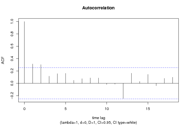
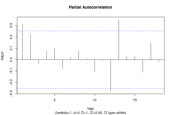
Title produced by software

(Partial) Autocorrelation Function

Date of computation

Fri, 09 Dec 2011 05:44:11 -0500

Cite this page as follows

Statistical Computations at FreeStatistics.org, Office for Research Development and Education, URL https://freestatistics.org/blog/index.php?v=date/2011/Dec/09/t13234274707ivt5mcsr1c1r6r.htm/, Retrieved Sun, 28 Apr 2024 16:50:42 +0000

Statistical Computations at FreeStatistics.org, Office for Research Development and Education, URL https://freestatistics.org/blog/index.php?pk=153246, Retrieved Sun, 28 Apr 2024 16:50:42 +0000

QR Codes:

Paste this QR Code to cite your computation.

Original text written by user:

IsPrivate?

No (this computation is public)

User-defined keywords

Estimated Impact

204

Family? (F = Feedback message, R = changed R code, M = changed R Module, P = changed Parameters, D = changed Data)

-     [Univariate Data Series] [] [2010-10-06 14:13:06] [3d53bd477a917086cfdff0f854c5e476]
-   PD  [Univariate Data Series] [rozen] [2010-12-07 20:04:29] [b98453cac15ba1066b407e146608df68]
- RMPD      [(Partial) Autocorrelation Function] [Times Series - Rozen] [2011-12-09 10:44:11] [a0aae37dd27f4b65e222573f53b5a13b] [Current]
- R P         [(Partial) Autocorrelation Function] [Times Series - Rozen] [2011-12-09 10:46:56] [586787d3e7267c593af3e1f6b16aa21a] 
- RMP         [Spectral Analysis] [Times Series] [2011-12-09 10:52:19] [586787d3e7267c593af3e1f6b16aa21a] 
- R P           [Spectral Analysis] [Times Series] [2011-12-09 10:53:58] [586787d3e7267c593af3e1f6b16aa21a] 
- R P           [Spectral Analysis] [Times Series] [2011-12-09 11:01:26] [586787d3e7267c593af3e1f6b16aa21a] 
- RMP           [Standard Deviation-Mean Plot] [Times Series] [2011-12-09 11:06:30] [586787d3e7267c593af3e1f6b16aa21a] 
- RMP           [ARIMA Backward Selection] [Times Series] [2011-12-09 11:19:36] [586787d3e7267c593af3e1f6b16aa21a] 
-    D            [ARIMA Backward Selection] [Arima] [2011-12-17 16:17:50] [f033824ca1b38a5ddbb2c3414ea3bb75] 
- RMPD            [Univariate Data Series] [Sterftegevallen p...] [2011-12-17 17:11:02] [f033824ca1b38a5ddbb2c3414ea3bb75] 
- RMPD            [Univariate Data Series] [aantal sterftegev...] [2011-12-17 17:22:01] [f033824ca1b38a5ddbb2c3414ea3bb75] 
- R  D              [Univariate Data Series] [Gemiddelde temp p...] [2011-12-17 17:23:28] [f033824ca1b38a5ddbb2c3414ea3bb75] 
- RMPD          [Maximum-likelihood Fitting - Normal Distribution] [Histogram Connected] [2011-12-09 12:22:17] [586787d3e7267c593af3e1f6b16aa21a] 
- RMPD          [Percentiles] [QQ Plot Connected] [2011-12-09 12:24:57] [586787d3e7267c593af3e1f6b16aa21a] 
- RMPD          [Tukey lambda PPCC Plot] [Tukey Connected] [2011-12-09 12:27:19] [586787d3e7267c593af3e1f6b16aa21a] 
- RMPD          [Skewness and Kurtosis Test] [Skewness-Kurtosis...] [2011-12-09 12:34:26] [586787d3e7267c593af3e1f6b16aa21a] 
- RMPD          [Maximum-likelihood Fitting - Normal Distribution] [Histogram - Seperate] [2011-12-09 12:48:43] [586787d3e7267c593af3e1f6b16aa21a] 
- RMPD          [Percentiles] [Q-Q Plot - Seperate] [2011-12-09 12:49:50] [586787d3e7267c593af3e1f6b16aa21a] 
- RMPD          [Tukey lambda PPCC Plot] [Tukey - Seperate] [2011-12-09 12:52:02] [586787d3e7267c593af3e1f6b16aa21a] 
- RMPD          [Skewness and Kurtosis Test] [Skewness/Kurtosis...] [2011-12-09 12:54:08] [586787d3e7267c593af3e1f6b16aa21a] 
- RMPD          [Central Tendency] [Median and Mean -...] [2011-12-09 13:03:03] [586787d3e7267c593af3e1f6b16aa21a] 
- R  D            [Central Tendency] [Mean and Median -...] [2011-12-09 13:12:15] [586787d3e7267c593af3e1f6b16aa21a] 

Feedback Forum

Post a new message

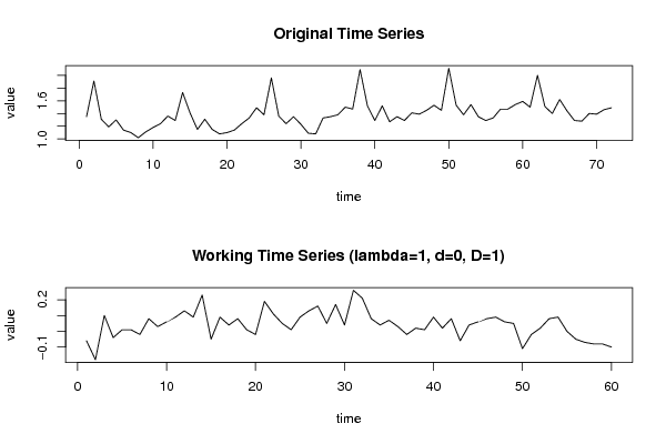
Dataseries X:

Download CSV

Histogram

Boxplots

1.35
1.91
1.31
1.19
1.3
1.14
1.1
1.02
1.11
1.18
1.24
1.36
1.29
1.73
1.41
1.15
1.31
1.15
1.08
1.1
1.14
1.24
1.33
1.49
1.38
1.96
1.36
1.24
1.35
1.23
1.09
1.08
1.33
1.35
1.38
1.5
1.47
2.09
1.52
1.29
1.52
1.27
1.35
1.29
1.41
1.39
1.45
1.53
1.45
2.11
1.53
1.38
1.54
1.35
1.29
1.33
1.47
1.47
1.54
1.59
1.5
2
1.51
1.4
1.62
1.44
1.29
1.28
1.4
1.39
1.46
1.49

Summary of computational transaction
Raw Input	view raw input (R code)
Raw Output	view raw output of R engine
Computing time	1 seconds
R Server	'George Udny Yule' @ yule.wessa.net

\begin{tabular}{lllllllll}
\hline
Summary of computational transaction \tabularnewline
Raw Input & view raw input (R code)  \tabularnewline
Raw Output & view raw output of R engine  \tabularnewline
Computing time & 1 seconds \tabularnewline
R Server & 'George Udny Yule' @ yule.wessa.net \tabularnewline
\hline
\end{tabular}
%Source: https://freestatistics.org/blog/index.php?pk=153246&T=0

[TABLE]
[ROW][C]Summary of computational transaction[/C][/ROW]
[ROW][C]Raw Input[/C][C]view raw input (R code) [/C][/ROW]
[ROW][C]Raw Output[/C][C]view raw output of R engine [/C][/ROW]
[ROW][C]Computing time[/C][C]1 seconds[/C][/ROW]
[ROW][C]R Server[/C][C]'George Udny Yule' @ yule.wessa.net[/C][/ROW]
[/TABLE]
Source: https://freestatistics.org/blog/index.php?pk=153246&T=0

Globally Unique Identifier (entire table): ba.freestatistics.org/blog/index.php?pk=153246&T=0

As an alternative you can also use a QR Code:

The GUIDs for individual cells are displayed in the table below:

Summary of computational transaction
Raw Input	view raw input (R code)
Raw Output	view raw output of R engine
Computing time	1 seconds
R Server	'George Udny Yule' @ yule.wessa.net

Autocorrelation Function
Time lag k	ACF(k)	T-STAT	P-value
1	0.312919	2.4239	0.009194
2	0.303151	2.3482	0.011089
3	0.115592	0.8954	0.187083
4	0.156506	1.2123	0.115077
5	0.161429	1.2504	0.108
6	0.048415	0.375	0.354484
7	0.075678	0.5862	0.279971
8	0.087958	0.6813	0.249146
9	0.086535	0.6703	0.25262
10	-0.018118	-0.1403	0.44443
11	-0.013059	-0.1012	0.459882
12	-0.245834	-1.9042	0.03084
13	0.163434	1.266	0.105211
14	0.030455	0.2359	0.407155
15	0.144774	1.1214	0.133289
16	-0.040222	-0.3116	0.378229
17	0.079715	0.6175	0.26963
18	0.098481	0.7628	0.224276

\begin{tabular}{lllllllll}
\hline
Autocorrelation Function \tabularnewline
Time lag k & ACF(k) & T-STAT & P-value \tabularnewline
1 & 0.312919 & 2.4239 & 0.009194 \tabularnewline
2 & 0.303151 & 2.3482 & 0.011089 \tabularnewline
3 & 0.115592 & 0.8954 & 0.187083 \tabularnewline
4 & 0.156506 & 1.2123 & 0.115077 \tabularnewline
5 & 0.161429 & 1.2504 & 0.108 \tabularnewline
6 & 0.048415 & 0.375 & 0.354484 \tabularnewline
7 & 0.075678 & 0.5862 & 0.279971 \tabularnewline
8 & 0.087958 & 0.6813 & 0.249146 \tabularnewline
9 & 0.086535 & 0.6703 & 0.25262 \tabularnewline
10 & -0.018118 & -0.1403 & 0.44443 \tabularnewline
11 & -0.013059 & -0.1012 & 0.459882 \tabularnewline
12 & -0.245834 & -1.9042 & 0.03084 \tabularnewline
13 & 0.163434 & 1.266 & 0.105211 \tabularnewline
14 & 0.030455 & 0.2359 & 0.407155 \tabularnewline
15 & 0.144774 & 1.1214 & 0.133289 \tabularnewline
16 & -0.040222 & -0.3116 & 0.378229 \tabularnewline
17 & 0.079715 & 0.6175 & 0.26963 \tabularnewline
18 & 0.098481 & 0.7628 & 0.224276 \tabularnewline
\hline
\end{tabular}
%Source: https://freestatistics.org/blog/index.php?pk=153246&T=1

[TABLE]
[ROW][C]Autocorrelation Function[/C][/ROW]
[ROW][C]Time lag k[/C][C]ACF(k)[/C][C]T-STAT[/C][C]P-value[/C][/ROW]
[ROW][C]1[/C][C]0.312919[/C][C]2.4239[/C][C]0.009194[/C][/ROW]
[ROW][C]2[/C][C]0.303151[/C][C]2.3482[/C][C]0.011089[/C][/ROW]
[ROW][C]3[/C][C]0.115592[/C][C]0.8954[/C][C]0.187083[/C][/ROW]
[ROW][C]4[/C][C]0.156506[/C][C]1.2123[/C][C]0.115077[/C][/ROW]
[ROW][C]5[/C][C]0.161429[/C][C]1.2504[/C][C]0.108[/C][/ROW]
[ROW][C]6[/C][C]0.048415[/C][C]0.375[/C][C]0.354484[/C][/ROW]
[ROW][C]7[/C][C]0.075678[/C][C]0.5862[/C][C]0.279971[/C][/ROW]
[ROW][C]8[/C][C]0.087958[/C][C]0.6813[/C][C]0.249146[/C][/ROW]
[ROW][C]9[/C][C]0.086535[/C][C]0.6703[/C][C]0.25262[/C][/ROW]
[ROW][C]10[/C][C]-0.018118[/C][C]-0.1403[/C][C]0.44443[/C][/ROW]
[ROW][C]11[/C][C]-0.013059[/C][C]-0.1012[/C][C]0.459882[/C][/ROW]
[ROW][C]12[/C][C]-0.245834[/C][C]-1.9042[/C][C]0.03084[/C][/ROW]
[ROW][C]13[/C][C]0.163434[/C][C]1.266[/C][C]0.105211[/C][/ROW]
[ROW][C]14[/C][C]0.030455[/C][C]0.2359[/C][C]0.407155[/C][/ROW]
[ROW][C]15[/C][C]0.144774[/C][C]1.1214[/C][C]0.133289[/C][/ROW]
[ROW][C]16[/C][C]-0.040222[/C][C]-0.3116[/C][C]0.378229[/C][/ROW]
[ROW][C]17[/C][C]0.079715[/C][C]0.6175[/C][C]0.26963[/C][/ROW]
[ROW][C]18[/C][C]0.098481[/C][C]0.7628[/C][C]0.224276[/C][/ROW]
[/TABLE]
Source: https://freestatistics.org/blog/index.php?pk=153246&T=1

Globally Unique Identifier (entire table): ba.freestatistics.org/blog/index.php?pk=153246&T=1

As an alternative you can also use a QR Code:

The GUIDs for individual cells are displayed in the table below:

Autocorrelation Function
Time lag k	ACF(k)	T-STAT	P-value
1	0.312919	2.4239	0.009194
2	0.303151	2.3482	0.011089
3	0.115592	0.8954	0.187083
4	0.156506	1.2123	0.115077
5	0.161429	1.2504	0.108
6	0.048415	0.375	0.354484
7	0.075678	0.5862	0.279971
8	0.087958	0.6813	0.249146
9	0.086535	0.6703	0.25262
10	-0.018118	-0.1403	0.44443
11	-0.013059	-0.1012	0.459882
12	-0.245834	-1.9042	0.03084
13	0.163434	1.266	0.105211
14	0.030455	0.2359	0.407155
15	0.144774	1.1214	0.133289
16	-0.040222	-0.3116	0.378229
17	0.079715	0.6175	0.26963
18	0.098481	0.7628	0.224276

Partial Autocorrelation Function
Time lag k	PACF(k)	T-STAT	P-value
1	0.312919	2.4239	0.009194
2	0.22751	1.7623	0.041557
3	-0.033762	-0.2615	0.397293
4	0.078179	0.6056	0.273542
5	0.104278	0.8077	0.211217
6	-0.077878	-0.6032	0.274311
7	0.022349	0.1731	0.431571
8	0.077776	0.6024	0.274573
9	0.009455	0.0732	0.470929
10	-0.104371	-0.8085	0.211012
11	-0.006019	-0.0466	0.481483
12	-0.275793	-2.1363	0.018372
13	0.351007	2.7189	0.004276
14	0.031132	0.2411	0.405132
15	0.03299	0.2555	0.399589
16	-0.110226	-0.8538	0.198304
17	0.143947	1.115	0.134646
18	-0.017793	-0.1378	0.445419

\begin{tabular}{lllllllll}
\hline
Partial Autocorrelation Function \tabularnewline
Time lag k & PACF(k) & T-STAT & P-value \tabularnewline
1 & 0.312919 & 2.4239 & 0.009194 \tabularnewline
2 & 0.22751 & 1.7623 & 0.041557 \tabularnewline
3 & -0.033762 & -0.2615 & 0.397293 \tabularnewline
4 & 0.078179 & 0.6056 & 0.273542 \tabularnewline
5 & 0.104278 & 0.8077 & 0.211217 \tabularnewline
6 & -0.077878 & -0.6032 & 0.274311 \tabularnewline
7 & 0.022349 & 0.1731 & 0.431571 \tabularnewline
8 & 0.077776 & 0.6024 & 0.274573 \tabularnewline
9 & 0.009455 & 0.0732 & 0.470929 \tabularnewline
10 & -0.104371 & -0.8085 & 0.211012 \tabularnewline
11 & -0.006019 & -0.0466 & 0.481483 \tabularnewline
12 & -0.275793 & -2.1363 & 0.018372 \tabularnewline
13 & 0.351007 & 2.7189 & 0.004276 \tabularnewline
14 & 0.031132 & 0.2411 & 0.405132 \tabularnewline
15 & 0.03299 & 0.2555 & 0.399589 \tabularnewline
16 & -0.110226 & -0.8538 & 0.198304 \tabularnewline
17 & 0.143947 & 1.115 & 0.134646 \tabularnewline
18 & -0.017793 & -0.1378 & 0.445419 \tabularnewline
\hline
\end{tabular}
%Source: https://freestatistics.org/blog/index.php?pk=153246&T=2

[TABLE]
[ROW][C]Partial Autocorrelation Function[/C][/ROW]
[ROW][C]Time lag k[/C][C]PACF(k)[/C][C]T-STAT[/C][C]P-value[/C][/ROW]
[ROW][C]1[/C][C]0.312919[/C][C]2.4239[/C][C]0.009194[/C][/ROW]
[ROW][C]2[/C][C]0.22751[/C][C]1.7623[/C][C]0.041557[/C][/ROW]
[ROW][C]3[/C][C]-0.033762[/C][C]-0.2615[/C][C]0.397293[/C][/ROW]
[ROW][C]4[/C][C]0.078179[/C][C]0.6056[/C][C]0.273542[/C][/ROW]
[ROW][C]5[/C][C]0.104278[/C][C]0.8077[/C][C]0.211217[/C][/ROW]
[ROW][C]6[/C][C]-0.077878[/C][C]-0.6032[/C][C]0.274311[/C][/ROW]
[ROW][C]7[/C][C]0.022349[/C][C]0.1731[/C][C]0.431571[/C][/ROW]
[ROW][C]8[/C][C]0.077776[/C][C]0.6024[/C][C]0.274573[/C][/ROW]
[ROW][C]9[/C][C]0.009455[/C][C]0.0732[/C][C]0.470929[/C][/ROW]
[ROW][C]10[/C][C]-0.104371[/C][C]-0.8085[/C][C]0.211012[/C][/ROW]
[ROW][C]11[/C][C]-0.006019[/C][C]-0.0466[/C][C]0.481483[/C][/ROW]
[ROW][C]12[/C][C]-0.275793[/C][C]-2.1363[/C][C]0.018372[/C][/ROW]
[ROW][C]13[/C][C]0.351007[/C][C]2.7189[/C][C]0.004276[/C][/ROW]
[ROW][C]14[/C][C]0.031132[/C][C]0.2411[/C][C]0.405132[/C][/ROW]
[ROW][C]15[/C][C]0.03299[/C][C]0.2555[/C][C]0.399589[/C][/ROW]
[ROW][C]16[/C][C]-0.110226[/C][C]-0.8538[/C][C]0.198304[/C][/ROW]
[ROW][C]17[/C][C]0.143947[/C][C]1.115[/C][C]0.134646[/C][/ROW]
[ROW][C]18[/C][C]-0.017793[/C][C]-0.1378[/C][C]0.445419[/C][/ROW]
[/TABLE]
Source: https://freestatistics.org/blog/index.php?pk=153246&T=2

Globally Unique Identifier (entire table): ba.freestatistics.org/blog/index.php?pk=153246&T=2

As an alternative you can also use a QR Code:

The GUIDs for individual cells are displayed in the table below:

Partial Autocorrelation Function
Time lag k	PACF(k)	T-STAT	P-value
1	0.312919	2.4239	0.009194
2	0.22751	1.7623	0.041557
3	-0.033762	-0.2615	0.397293
4	0.078179	0.6056	0.273542
5	0.104278	0.8077	0.211217
6	-0.077878	-0.6032	0.274311
7	0.022349	0.1731	0.431571
8	0.077776	0.6024	0.274573
9	0.009455	0.0732	0.470929
10	-0.104371	-0.8085	0.211012
11	-0.006019	-0.0466	0.481483
12	-0.275793	-2.1363	0.018372
13	0.351007	2.7189	0.004276
14	0.031132	0.2411	0.405132
15	0.03299	0.2555	0.399589
16	-0.110226	-0.8538	0.198304
17	0.143947	1.115	0.134646
18	-0.017793	-0.1378	0.445419

Figure 1

PNG link

Postscript link

PDF link

Figure 2

PNG link

Postscript link

PDF link

Figure 3

PNG link

Postscript link

PDF link

Parameters (Session):

par1 = Default ; par2 = 1 ; par3 = 0 ; par4 = 1 ; par5 = 12 ; par6 = White Noise ; par7 = 0.95 ;

Parameters (R input):

par1 = Default ; par2 = 1 ; par3 = 0 ; par4 = 1 ; par5 = 12 ; par6 = White Noise ; par7 = 0.95 ; par8 = ;

R code (references can be found in the software module):

if (par1 == 'Default') {
par1 = 10*log10(length(x))
} else {
par1 <- as.numeric(par1)
}
par2 <- as.numeric(par2)
par3 <- as.numeric(par3)
par4 <- as.numeric(par4)
par5 <- as.numeric(par5)
if (par6 == 'White Noise') par6 <- 'white' else par6 <- 'ma'
par7 <- as.numeric(par7)
if (par8 != '') par8 <- as.numeric(par8)
ox <- x
if (par8 == '') {
if (par2 == 0) {
x <- log(x)
} else {
x <- (x ^ par2 - 1) / par2
}
} else {
x <- log(x,base=par8)
}
if (par3 > 0) x <- diff(x,lag=1,difference=par3)
if (par4 > 0) x <- diff(x,lag=par5,difference=par4)
bitmap(file='picts.png')
op <- par(mfrow=c(2,1))
plot(ox,type='l',main='Original Time Series',xlab='time',ylab='value')
if (par8=='') {
mytitle <- paste('Working Time Series (lambda=',par2,', d=',par3,', D=',par4,')',sep='')
mysub <- paste('(lambda=',par2,', d=',par3,', D=',par4,', CI=', par7, ', CI type=',par6,')',sep='')
} else {
mytitle <- paste('Working Time Series (base=',par8,', d=',par3,', D=',par4,')',sep='')
mysub <- paste('(base=',par8,', d=',par3,', D=',par4,', CI=', par7, ', CI type=',par6,')',sep='')
}
plot(x,type='l', main=mytitle,xlab='time',ylab='value')
par(op)
dev.off()
bitmap(file='pic1.png')
racf <- acf(x, par1, main='Autocorrelation', xlab='time lag', ylab='ACF', ci.type=par6, ci=par7, sub=mysub)
dev.off()
bitmap(file='pic2.png')
rpacf <- pacf(x,par1,main='Partial Autocorrelation',xlab='lags',ylab='PACF',sub=mysub)
dev.off()
(myacf <- c(racf$acf))
(mypacf <- c(rpacf$acf))
lengthx <- length(x)
sqrtn <- sqrt(lengthx)
load(file='createtable')
a<-table.start()
a<-table.row.start(a)
a<-table.element(a,'Autocorrelation Function',4,TRUE)
a<-table.row.end(a)
a<-table.row.start(a)
a<-table.element(a,'Time lag k',header=TRUE)
a<-table.element(a,hyperlink('basics.htm','ACF(k)','click here for more information about the Autocorrelation Function'),header=TRUE)
a<-table.element(a,'T-STAT',header=TRUE)
a<-table.element(a,'P-value',header=TRUE)
a<-table.row.end(a)
for (i in 2:(par1+1)) {
a<-table.row.start(a)
a<-table.element(a,i-1,header=TRUE)
a<-table.element(a,round(myacf[i],6))
mytstat <- myacf[i]*sqrtn
a<-table.element(a,round(mytstat,4))
a<-table.element(a,round(1-pt(abs(mytstat),lengthx),6))
a<-table.row.end(a)
}
a<-table.end(a)
table.save(a,file='mytable.tab')
a<-table.start()
a<-table.row.start(a)
a<-table.element(a,'Partial Autocorrelation Function',4,TRUE)
a<-table.row.end(a)
a<-table.row.start(a)
a<-table.element(a,'Time lag k',header=TRUE)
a<-table.element(a,hyperlink('basics.htm','PACF(k)','click here for more information about the Partial Autocorrelation Function'),header=TRUE)
a<-table.element(a,'T-STAT',header=TRUE)
a<-table.element(a,'P-value',header=TRUE)
a<-table.row.end(a)
for (i in 1:par1) {
a<-table.row.start(a)
a<-table.element(a,i,header=TRUE)
a<-table.element(a,round(mypacf[i],6))
mytstat <- mypacf[i]*sqrtn
a<-table.element(a,round(mytstat,4))
a<-table.element(a,round(1-pt(abs(mytstat),lengthx),6))
a<-table.row.end(a)
}
a<-table.end(a)
table.save(a,file='mytable1.tab')

Free Statistics

Description of Statistical Computation

Tree of Dependent Computations

Dataset

Tables (Output of Computation)

Figures (Output of Computation)

Input Parameters & R Code