Repository of Reproducible Computations

Free Statistics

of Irreproducible Research!

Author's title

Author

*The author of this computation has been verified*

R Software Module

rwasp_Two Factor ANOVA.wasp

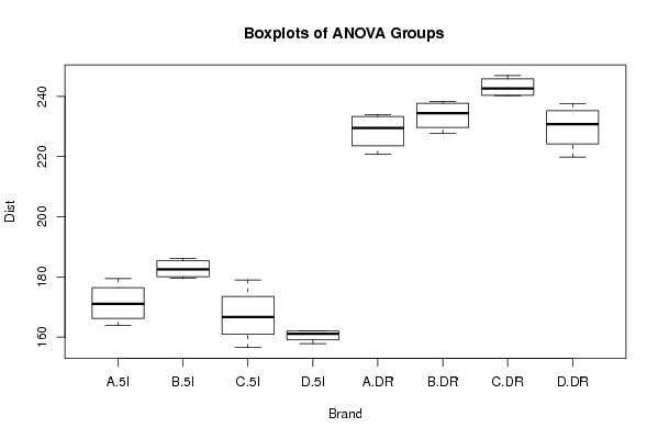
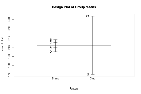
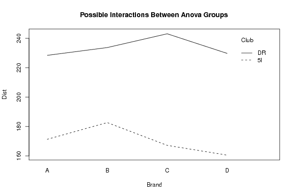
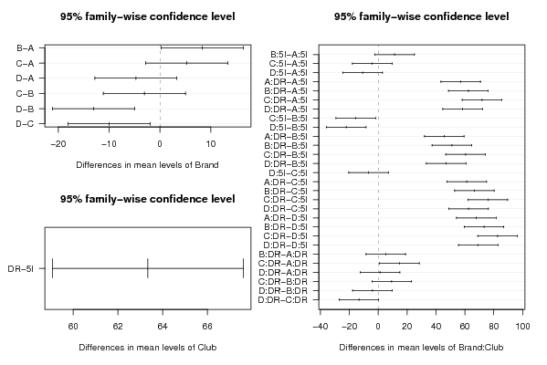
Title produced by software

Two-Way ANOVA

Date of computation

Mon, 25 Oct 2010 12:43:22 +0000

Cite this page as follows

Statistical Computations at FreeStatistics.org, Office for Research Development and Education, URL https://freestatistics.org/blog/index.php?v=date/2010/Oct/25/t1288010724vna3s9frpmr7kly.htm/, Retrieved Mon, 29 Apr 2024 13:40:45 +0000

Statistical Computations at FreeStatistics.org, Office for Research Development and Education, URL https://freestatistics.org/blog/index.php?pk=88094, Retrieved Mon, 29 Apr 2024 13:40:45 +0000

QR Codes:

Paste this QR Code to cite your computation.

Original text written by user:

IsPrivate?

No (this computation is public)

User-defined keywords

Estimated Impact

351

Family? (F = Feedback message, R = changed R code, M = changed R Module, P = changed Parameters, D = changed Data)

-       [Two-Way ANOVA] [Golfballs] [2010-10-25 12:43:22] [d76b387543b13b5e3afd8ff9e5fdc89f] [Current]
-   PD    [Two-Way ANOVA] [WS5: Vraag 8] [2010-10-29 09:31:50] [1fd136673b2a4fecb5c545b9b4a05d64] 
-   PD      [Two-Way ANOVA] [Workshop 5 - Q8] [2010-10-29 13:53:54] [6f0e7a2d1a07390e3505a2db8288f975] 
F   P         [Two-Way ANOVA] [Taak 8: two way A...] [2010-10-29 14:11:06] [74deae64b71f9d77c839af86f7c687b5] 
F    D          [Two-Way ANOVA] [WS5 Q8] [2010-11-02 12:05:39] [afe9379cca749d06b3d6872e02cc47ed] 
- R PD            [Two-Way ANOVA] [WS 5 - Q8] [2010-11-02 15:15:23] [18fa53e8b37a5effc0c5f8a5122cdd2d] 
F   PD            [Two-Way ANOVA] [] [2010-11-02 15:16:56] [fc9068db680cd880760a7c0fccd81a61] 
- RMPD            [Paired and Unpaired Two Samples Tests about the Mean] [W5 - correction 2] [2010-11-08 19:17:28] [48146708a479232c43a8f6e52fbf83b4] 
- RMPD            [Paired and Unpaired Two Samples Tests about the Mean] [W5 - correction 1] [2010-11-08 19:19:44] [48146708a479232c43a8f6e52fbf83b4] 
- RMPD            [Paired and Unpaired Two Samples Tests about the Mean] [W5 - correction 3] [2010-11-08 19:21:37] [48146708a479232c43a8f6e52fbf83b4] 
- RMPD            [Paired and Unpaired Two Samples Tests about the Mean] [W5 - correction 5(E)] [2010-11-08 19:26:42] [48146708a479232c43a8f6e52fbf83b4] 
- RMPD            [Paired and Unpaired Two Samples Tests about the Mean] [W5 - correction 5(T)] [2010-11-08 19:28:24] [48146708a479232c43a8f6e52fbf83b4] 
- RMPD            [Paired and Unpaired Two Samples Tests about the Mean] [W5 - correction 5(S)] [2010-11-08 19:30:16] [48146708a479232c43a8f6e52fbf83b4] 
- R               [Two-Way ANOVA] [WS5 _- Q8 ] [2011-11-08 22:17:05] [2c786c21adba4dd4c8af44dce5258f06] 
- R P             [Two-Way ANOVA] [ws 5 - opdracht 8] [2011-11-08 22:46:01] [4b648d52023f19d55c572f0eddd72b1f] 
- RM              [Two-Way ANOVA] [Question 8] [2012-10-29 16:10:27] [4bcde15d59f799c0000a3f03b8626620] 
- R P             [Two-Way ANOVA] [WS5 taak 8] [2012-10-29 17:26:40] [ebc10d82be597731a57172229e4f44b7] 
- R P             [Two-Way ANOVA] [Q8] [2012-10-29 21:23:10] [74be16979710d4c4e7c6647856088456] 
- R PD            [Two-Way ANOVA] [WS 5 Q 8] [2012-10-30 09:57:08] [8c30f4dd45e15fd207e4faf2fdf6253e] 
- R P               [Two-Way ANOVA] [Paper - 2-way anova] [2012-12-19 18:54:42] [7dcdf88f8d4909016d1a598b3c226ce5] 
- R P               [Two-Way ANOVA] [Paper - 2 way ano...] [2012-12-19 18:51:42] [7dcdf88f8d4909016d1a598b3c226ce5] 
- R P               [Two-Way ANOVA] [] [2012-12-20 23:48:25] [a4b60d76ea6b846adbf54f7861413bce] 
-           [Two-Way ANOVA] [ws5.8] [2010-11-01 13:47:19] [e4076051fbfb461c886b1e223cd7862f] 
- R  D      [Two-Way ANOVA] [WS5- Task 8] [2010-11-02 12:31:34] [19f9551d4d95750ef21e9f3cf8fe2131] 
-    D        [Two-Way ANOVA] [p_Stress_Anova1] [2010-12-04 12:16:48] [19f9551d4d95750ef21e9f3cf8fe2131] 
-               [Two-Way ANOVA] [p_Stress_Anova1] [2010-12-04 12:25:19] [19f9551d4d95750ef21e9f3cf8fe2131] 
- R           [Two-Way ANOVA] [] [2011-11-06 10:58:56] [74be16979710d4c4e7c6647856088456] 
- RM          [Two-Way ANOVA] [] [2011-11-06 21:01:21] [74be16979710d4c4e7c6647856088456] 
-   PD      [Two-Way ANOVA] [question 8] [2010-11-02 13:33:25] [dc30d19c3bc2be07fe595ad36c2cf923] 
- R  D      [Two-Way ANOVA] [Q8] [2010-11-02 18:32:47] [8ec018d7298e4a3ae278d8b7199e08b6] 
- R         [Two-Way ANOVA] [WS 5 Question 8] [2011-11-01 19:56:50] [f5fdea4413921432bb019d1f20c4f2ec] 
- R         [Two-Way ANOVA] [Q8] [2011-11-05 14:06:39] [9e469a83342941fcd5c6dffbf184cd3a] 
- RM        [Two-Way ANOVA] [] [2011-11-08 19:10:23] [74be16979710d4c4e7c6647856088456] 
F   PD    [Two-Way ANOVA] [W5 Q8] [2010-10-29 12:39:31] [56d90b683fcd93137645f9226b43c62b] 
-   PD    [Two-Way ANOVA] [question 8] [2010-10-29 13:51:27] [c1605865773cc027e55b238d879a644c] 
-   P       [Two-Way ANOVA] [] [2010-11-01 10:17:22] [22937c5b58c14f6c22964f32d64ff823] 
F   P         [Two-Way ANOVA] [workshop 5 Questi...] [2010-11-01 16:13:46] [945bcebba5e7ac34a41d6888338a1ba9] 
-   P           [Two-Way ANOVA] [] [2010-11-02 14:54:17] [5278e0a58c5de897b31ce79607e774d7] 
-   P         [Two-Way ANOVA] [workshop 8] [2010-11-02 15:14:13] [8d09066a9d3795298da6860e7d4a4400] 
F           [Two-Way ANOVA] [WS5 Q8] [2010-11-02 13:18:31] [3b4d50908b02f70d585ba4c3ab01ca98] 
-   P         [Two-Way ANOVA] [vraag 8] [2010-11-02 13:58:05] [717f3d787904f94c39256c5c1fc72d4c] 
- R PD      [Two-Way ANOVA] [Question 8] [2010-11-02 13:47:52] [13c73ac943380855a1c72833078e44d2] 
-             [Two-Way ANOVA] [] [2010-11-03 13:01:24] [43239ed98a62e091c70785d80176537f] 
- R PD      [Two-Way ANOVA] [Workshop 5 - Ques...] [2010-11-02 16:19:28] [74be16979710d4c4e7c6647856088456] 
F   P         [Two-Way ANOVA] [Question 8 Expirm...] [2010-11-02 17:39:46] [d59201e34006b7e3f71c33fa566f42b3] 
-   PD    [Two-Way ANOVA] [workshop 5 - taak 8] [2010-10-29 13:52:18] [956e8df26b41c50d9c6c2ec1b6a122a8] 
-   PD    [Two-Way ANOVA] [Question 8] [2010-10-29 13:51:31] [2960375a246cc0628590c95c4038a43c] 
-   PD    [Two-Way ANOVA] [Vraag 8] [2010-10-29 13:52:04] [d7a673bc47e3999e70f4e1e2276e5189] 
-           [Two-Way ANOVA] [Workshop 5: Quest...] [2010-10-30 12:18:25] [62f7c80c4d96454bbd2b2b026ea9aad9] 

[Truncated]

Feedback Forum

Post a new message

Dataseries X:

Download CSV

Histogram

Boxplots

226.4	'A'	'DR'
232.6	'A'	'DR'
234	'A'	'DR'
220.7	'A'	'DR'
163.8	'A'	'5I'
179.4	'A'	'5I'
168.6	'A'	'5I'
173.4	'A'	'5I'
238.3	'B'	'DR'
231.7	'B'	'DR'
227.7	'B'	'DR'
237.2	'B'	'DR'
184.4	'B'	'5I'
180.6	'B'	'5I'
179.5	'B'	'5I'
186.2	'B'	'5I'
240.5	'C'	'DR'
246.9	'C'	'DR'
240.3	'C'	'DR'
244.7	'C'	'DR'
179	'C'	'5I'
168	'C'	'5I'
165.2	'C'	'5I'
156.5	'C'	'5I'
219.8	'D'	'DR'
228.7	'D'	'DR'
232.9	'D'	'DR'
237.6	'D'	'DR'
157.8	'D'	'5I'
161.8	'D'	'5I'
162.1	'D'	'5I'
160.3	'D'	'5I'

Summary of computational transaction
Raw Input	view raw input (R code)
Raw Output	view raw output of R engine
Computing time	2 seconds
R Server	'Gwilym Jenkins' @ 72.249.127.135

\begin{tabular}{lllllllll}
\hline
Summary of computational transaction \tabularnewline
Raw Input & view raw input (R code)  \tabularnewline
Raw Output & view raw output of R engine  \tabularnewline
Computing time & 2 seconds \tabularnewline
R Server & 'Gwilym Jenkins' @ 72.249.127.135 \tabularnewline
\hline
\end{tabular}
%Source: https://freestatistics.org/blog/index.php?pk=88094&T=0

[TABLE]
[ROW][C]Summary of computational transaction[/C][/ROW]
[ROW][C]Raw Input[/C][C]view raw input (R code) [/C][/ROW]
[ROW][C]Raw Output[/C][C]view raw output of R engine [/C][/ROW]
[ROW][C]Computing time[/C][C]2 seconds[/C][/ROW]
[ROW][C]R Server[/C][C]'Gwilym Jenkins' @ 72.249.127.135[/C][/ROW]
[/TABLE]
Source: https://freestatistics.org/blog/index.php?pk=88094&T=0

Globally Unique Identifier (entire table): ba.freestatistics.org/blog/index.php?pk=88094&T=0

As an alternative you can also use a QR Code:

The GUIDs for individual cells are displayed in the table below:

Summary of computational transaction
Raw Input	view raw input (R code)
Raw Output	view raw output of R engine
Computing time	2 seconds
R Server	'Gwilym Jenkins' @ 72.249.127.135

ANOVA Model
Response ~ Treatment_A * Treatment_B
means	171.3	11.375	-4.125	-10.8	57.125	-6.075	18.8	12.125

\begin{tabular}{lllllllll}
\hline
ANOVA Model \tabularnewline
Response ~ Treatment_A * Treatment_B \tabularnewline
means & 171.3 & 11.375 & -4.125 & -10.8 & 57.125 & -6.075 & 18.8 & 12.125 \tabularnewline
\hline
\end{tabular}
%Source: https://freestatistics.org/blog/index.php?pk=88094&T=1

[TABLE]
[ROW][C]ANOVA Model[/C][/ROW]
[ROW][C]Response ~ Treatment_A * Treatment_B[/C][/ROW]
[ROW][C]means[/C][C]171.3[/C][C]11.375[/C][C]-4.125[/C][C]-10.8[/C][C]57.125[/C][C]-6.075[/C][C]18.8[/C][C]12.125[/C][/ROW]
[/TABLE]
Source: https://freestatistics.org/blog/index.php?pk=88094&T=1

Globally Unique Identifier (entire table): ba.freestatistics.org/blog/index.php?pk=88094&T=1

As an alternative you can also use a QR Code:

The GUIDs for individual cells are displayed in the table below:

ANOVA Model
Response ~ Treatment_A * Treatment_B
means	171.3	11.375	-4.125	-10.8	57.125	-6.075	18.8	12.125

ANOVA Statistics
	Df	Sum Sq	Mean Sq	F value	Pr(>F)
	3
Treatment_A	3	800.736	266.912	7.791	0.001
Treatment_B	3	32093.111	32093.111	936.752	0
Treatment_A:Treatment_B	3	765.961	255.32	7.452	0.001
Residuals	24	822.24	34.26

\begin{tabular}{lllllllll}
\hline
ANOVA Statistics \tabularnewline
  & Df & Sum Sq & Mean Sq & F value & Pr(>F) \tabularnewline
 & 3 &  &  &  &  \tabularnewline
Treatment_A & 3 & 800.736 & 266.912 & 7.791 & 0.001 \tabularnewline
Treatment_B & 3 & 32093.111 & 32093.111 & 936.752 & 0 \tabularnewline
Treatment_A:Treatment_B & 3 & 765.961 & 255.32 & 7.452 & 0.001 \tabularnewline
Residuals & 24 & 822.24 & 34.26 &   &   \tabularnewline
\hline
\end{tabular}
%Source: https://freestatistics.org/blog/index.php?pk=88094&T=2

[TABLE]
[ROW][C]ANOVA Statistics[/C][/ROW]
[ROW][C] [/C][C]Df[/C][C]Sum Sq[/C][C]Mean Sq[/C][C]F value[/C][C]Pr(>F)[/C][/ROW]
[ROW][C][/C][C]3[/C][C][/C][C][/C][C][/C][C][/C][/ROW]
[ROW][C]Treatment_A[/C][C]3[/C][C]800.736[/C][C]266.912[/C][C]7.791[/C][C]0.001[/C][/ROW]
[ROW][C]Treatment_B[/C][C]3[/C][C]32093.111[/C][C]32093.111[/C][C]936.752[/C][C]0[/C][/ROW]
[ROW][C]Treatment_A:Treatment_B[/C][C]3[/C][C]765.961[/C][C]255.32[/C][C]7.452[/C][C]0.001[/C][/ROW]
[ROW][C]Residuals[/C][C]24[/C][C]822.24[/C][C]34.26[/C][C] [/C][C] [/C][/ROW]
[/TABLE]
Source: https://freestatistics.org/blog/index.php?pk=88094&T=2

Globally Unique Identifier (entire table): ba.freestatistics.org/blog/index.php?pk=88094&T=2

As an alternative you can also use a QR Code:

The GUIDs for individual cells are displayed in the table below:

ANOVA Statistics
	Df	Sum Sq	Mean Sq	F value	Pr(>F)
	3
Treatment_A	3	800.736	266.912	7.791	0.001
Treatment_B	3	32093.111	32093.111	936.752	0
Treatment_A:Treatment_B	3	765.961	255.32	7.452	0.001
Residuals	24	822.24	34.26

Tukey Honest Significant Difference Comparisons
	diff	lwr	upr	p adj
B-A	8.338	0.264	16.411	0.041
C-A	5.275	-2.798	13.348	0.297
D-A	-4.737	-12.811	3.336	0.387
C-B	-3.062	-11.136	5.011	0.724
D-B	-13.075	-21.148	-5.002	0.001
D-C	-10.012	-18.086	-1.939	0.011
DR-5I	63.337	59.066	67.609	0
B:5I-A:5I	11.375	-2.332	25.082	0.156
C:5I-A:5I	-4.125	-17.832	9.582	0.971
D:5I-A:5I	-10.8	-24.507	2.907	0.201
A:DR-A:5I	57.125	43.418	70.832	0
B:DR-A:5I	62.425	48.718	76.132	0
C:DR-A:5I	71.8	58.093	85.507	0
D:DR-A:5I	58.45	44.743	72.157	0
C:5I-B:5I	-15.5	-29.207	-1.793	0.019
D:5I-B:5I	-22.175	-35.882	-8.468	0
A:DR-B:5I	45.75	32.043	59.457	0
B:DR-B:5I	51.05	37.343	64.757	0
C:DR-B:5I	60.425	46.718	74.132	0
D:DR-B:5I	47.075	33.368	60.782	0
D:5I-C:5I	-6.675	-20.382	7.032	0.739
A:DR-C:5I	61.25	47.543	74.957	0
B:DR-C:5I	66.55	52.843	80.257	0
C:DR-C:5I	75.925	62.218	89.632	0
D:DR-C:5I	62.575	48.868	76.282	0
A:DR-D:5I	67.925	54.218	81.632	0
B:DR-D:5I	73.225	59.518	86.932	0
C:DR-D:5I	82.6	68.893	96.307	0
D:DR-D:5I	69.25	55.543	82.957	0
B:DR-A:DR	5.3	-8.407	19.007	0.897
C:DR-A:DR	14.675	0.968	28.382	0.03
D:DR-A:DR	1.325	-12.382	15.032	1
C:DR-B:DR	9.375	-4.332	23.082	0.351
D:DR-B:DR	-3.975	-17.682	9.732	0.976
D:DR-C:DR	-13.35	-27.057	0.357	0.06

\begin{tabular}{lllllllll}
\hline
Tukey Honest Significant Difference Comparisons \tabularnewline
  & diff & lwr & upr & p adj \tabularnewline
B-A & 8.338 & 0.264 & 16.411 & 0.041 \tabularnewline
C-A & 5.275 & -2.798 & 13.348 & 0.297 \tabularnewline
D-A & -4.737 & -12.811 & 3.336 & 0.387 \tabularnewline
C-B & -3.062 & -11.136 & 5.011 & 0.724 \tabularnewline
D-B & -13.075 & -21.148 & -5.002 & 0.001 \tabularnewline
D-C & -10.012 & -18.086 & -1.939 & 0.011 \tabularnewline
DR-5I & 63.337 & 59.066 & 67.609 & 0 \tabularnewline
B:5I-A:5I & 11.375 & -2.332 & 25.082 & 0.156 \tabularnewline
C:5I-A:5I & -4.125 & -17.832 & 9.582 & 0.971 \tabularnewline
D:5I-A:5I & -10.8 & -24.507 & 2.907 & 0.201 \tabularnewline
A:DR-A:5I & 57.125 & 43.418 & 70.832 & 0 \tabularnewline
B:DR-A:5I & 62.425 & 48.718 & 76.132 & 0 \tabularnewline
C:DR-A:5I & 71.8 & 58.093 & 85.507 & 0 \tabularnewline
D:DR-A:5I & 58.45 & 44.743 & 72.157 & 0 \tabularnewline
C:5I-B:5I & -15.5 & -29.207 & -1.793 & 0.019 \tabularnewline
D:5I-B:5I & -22.175 & -35.882 & -8.468 & 0 \tabularnewline
A:DR-B:5I & 45.75 & 32.043 & 59.457 & 0 \tabularnewline
B:DR-B:5I & 51.05 & 37.343 & 64.757 & 0 \tabularnewline
C:DR-B:5I & 60.425 & 46.718 & 74.132 & 0 \tabularnewline
D:DR-B:5I & 47.075 & 33.368 & 60.782 & 0 \tabularnewline
D:5I-C:5I & -6.675 & -20.382 & 7.032 & 0.739 \tabularnewline
A:DR-C:5I & 61.25 & 47.543 & 74.957 & 0 \tabularnewline
B:DR-C:5I & 66.55 & 52.843 & 80.257 & 0 \tabularnewline
C:DR-C:5I & 75.925 & 62.218 & 89.632 & 0 \tabularnewline
D:DR-C:5I & 62.575 & 48.868 & 76.282 & 0 \tabularnewline
A:DR-D:5I & 67.925 & 54.218 & 81.632 & 0 \tabularnewline
B:DR-D:5I & 73.225 & 59.518 & 86.932 & 0 \tabularnewline
C:DR-D:5I & 82.6 & 68.893 & 96.307 & 0 \tabularnewline
D:DR-D:5I & 69.25 & 55.543 & 82.957 & 0 \tabularnewline
B:DR-A:DR & 5.3 & -8.407 & 19.007 & 0.897 \tabularnewline
C:DR-A:DR & 14.675 & 0.968 & 28.382 & 0.03 \tabularnewline
D:DR-A:DR & 1.325 & -12.382 & 15.032 & 1 \tabularnewline
C:DR-B:DR & 9.375 & -4.332 & 23.082 & 0.351 \tabularnewline
D:DR-B:DR & -3.975 & -17.682 & 9.732 & 0.976 \tabularnewline
D:DR-C:DR & -13.35 & -27.057 & 0.357 & 0.06 \tabularnewline
\hline
\end{tabular}
%Source: https://freestatistics.org/blog/index.php?pk=88094&T=3

[TABLE]
[ROW][C]Tukey Honest Significant Difference Comparisons[/C][/ROW]
[ROW][C] [/C][C]diff[/C][C]lwr[/C][C]upr[/C][C]p adj[/C][/ROW]
[ROW][C]B-A[/C][C]8.338[/C][C]0.264[/C][C]16.411[/C][C]0.041[/C][/ROW]
[ROW][C]C-A[/C][C]5.275[/C][C]-2.798[/C][C]13.348[/C][C]0.297[/C][/ROW]
[ROW][C]D-A[/C][C]-4.737[/C][C]-12.811[/C][C]3.336[/C][C]0.387[/C][/ROW]
[ROW][C]C-B[/C][C]-3.062[/C][C]-11.136[/C][C]5.011[/C][C]0.724[/C][/ROW]
[ROW][C]D-B[/C][C]-13.075[/C][C]-21.148[/C][C]-5.002[/C][C]0.001[/C][/ROW]
[ROW][C]D-C[/C][C]-10.012[/C][C]-18.086[/C][C]-1.939[/C][C]0.011[/C][/ROW]
[ROW][C]DR-5I[/C][C]63.337[/C][C]59.066[/C][C]67.609[/C][C]0[/C][/ROW]
[ROW][C]B:5I-A:5I[/C][C]11.375[/C][C]-2.332[/C][C]25.082[/C][C]0.156[/C][/ROW]
[ROW][C]C:5I-A:5I[/C][C]-4.125[/C][C]-17.832[/C][C]9.582[/C][C]0.971[/C][/ROW]
[ROW][C]D:5I-A:5I[/C][C]-10.8[/C][C]-24.507[/C][C]2.907[/C][C]0.201[/C][/ROW]
[ROW][C]A:DR-A:5I[/C][C]57.125[/C][C]43.418[/C][C]70.832[/C][C]0[/C][/ROW]
[ROW][C]B:DR-A:5I[/C][C]62.425[/C][C]48.718[/C][C]76.132[/C][C]0[/C][/ROW]
[ROW][C]C:DR-A:5I[/C][C]71.8[/C][C]58.093[/C][C]85.507[/C][C]0[/C][/ROW]
[ROW][C]D:DR-A:5I[/C][C]58.45[/C][C]44.743[/C][C]72.157[/C][C]0[/C][/ROW]
[ROW][C]C:5I-B:5I[/C][C]-15.5[/C][C]-29.207[/C][C]-1.793[/C][C]0.019[/C][/ROW]
[ROW][C]D:5I-B:5I[/C][C]-22.175[/C][C]-35.882[/C][C]-8.468[/C][C]0[/C][/ROW]
[ROW][C]A:DR-B:5I[/C][C]45.75[/C][C]32.043[/C][C]59.457[/C][C]0[/C][/ROW]
[ROW][C]B:DR-B:5I[/C][C]51.05[/C][C]37.343[/C][C]64.757[/C][C]0[/C][/ROW]
[ROW][C]C:DR-B:5I[/C][C]60.425[/C][C]46.718[/C][C]74.132[/C][C]0[/C][/ROW]
[ROW][C]D:DR-B:5I[/C][C]47.075[/C][C]33.368[/C][C]60.782[/C][C]0[/C][/ROW]
[ROW][C]D:5I-C:5I[/C][C]-6.675[/C][C]-20.382[/C][C]7.032[/C][C]0.739[/C][/ROW]
[ROW][C]A:DR-C:5I[/C][C]61.25[/C][C]47.543[/C][C]74.957[/C][C]0[/C][/ROW]
[ROW][C]B:DR-C:5I[/C][C]66.55[/C][C]52.843[/C][C]80.257[/C][C]0[/C][/ROW]
[ROW][C]C:DR-C:5I[/C][C]75.925[/C][C]62.218[/C][C]89.632[/C][C]0[/C][/ROW]
[ROW][C]D:DR-C:5I[/C][C]62.575[/C][C]48.868[/C][C]76.282[/C][C]0[/C][/ROW]
[ROW][C]A:DR-D:5I[/C][C]67.925[/C][C]54.218[/C][C]81.632[/C][C]0[/C][/ROW]
[ROW][C]B:DR-D:5I[/C][C]73.225[/C][C]59.518[/C][C]86.932[/C][C]0[/C][/ROW]
[ROW][C]C:DR-D:5I[/C][C]82.6[/C][C]68.893[/C][C]96.307[/C][C]0[/C][/ROW]
[ROW][C]D:DR-D:5I[/C][C]69.25[/C][C]55.543[/C][C]82.957[/C][C]0[/C][/ROW]
[ROW][C]B:DR-A:DR[/C][C]5.3[/C][C]-8.407[/C][C]19.007[/C][C]0.897[/C][/ROW]
[ROW][C]C:DR-A:DR[/C][C]14.675[/C][C]0.968[/C][C]28.382[/C][C]0.03[/C][/ROW]
[ROW][C]D:DR-A:DR[/C][C]1.325[/C][C]-12.382[/C][C]15.032[/C][C]1[/C][/ROW]
[ROW][C]C:DR-B:DR[/C][C]9.375[/C][C]-4.332[/C][C]23.082[/C][C]0.351[/C][/ROW]
[ROW][C]D:DR-B:DR[/C][C]-3.975[/C][C]-17.682[/C][C]9.732[/C][C]0.976[/C][/ROW]
[ROW][C]D:DR-C:DR[/C][C]-13.35[/C][C]-27.057[/C][C]0.357[/C][C]0.06[/C][/ROW]
[/TABLE]
Source: https://freestatistics.org/blog/index.php?pk=88094&T=3

Globally Unique Identifier (entire table): ba.freestatistics.org/blog/index.php?pk=88094&T=3

As an alternative you can also use a QR Code:

The GUIDs for individual cells are displayed in the table below:

Tukey Honest Significant Difference Comparisons
	diff	lwr	upr	p adj
B-A	8.338	0.264	16.411	0.041
C-A	5.275	-2.798	13.348	0.297
D-A	-4.737	-12.811	3.336	0.387
C-B	-3.062	-11.136	5.011	0.724
D-B	-13.075	-21.148	-5.002	0.001
D-C	-10.012	-18.086	-1.939	0.011
DR-5I	63.337	59.066	67.609	0
B:5I-A:5I	11.375	-2.332	25.082	0.156
C:5I-A:5I	-4.125	-17.832	9.582	0.971
D:5I-A:5I	-10.8	-24.507	2.907	0.201
A:DR-A:5I	57.125	43.418	70.832	0
B:DR-A:5I	62.425	48.718	76.132	0
C:DR-A:5I	71.8	58.093	85.507	0
D:DR-A:5I	58.45	44.743	72.157	0
C:5I-B:5I	-15.5	-29.207	-1.793	0.019
D:5I-B:5I	-22.175	-35.882	-8.468	0
A:DR-B:5I	45.75	32.043	59.457	0
B:DR-B:5I	51.05	37.343	64.757	0
C:DR-B:5I	60.425	46.718	74.132	0
D:DR-B:5I	47.075	33.368	60.782	0
D:5I-C:5I	-6.675	-20.382	7.032	0.739
A:DR-C:5I	61.25	47.543	74.957	0
B:DR-C:5I	66.55	52.843	80.257	0
C:DR-C:5I	75.925	62.218	89.632	0
D:DR-C:5I	62.575	48.868	76.282	0
A:DR-D:5I	67.925	54.218	81.632	0
B:DR-D:5I	73.225	59.518	86.932	0
C:DR-D:5I	82.6	68.893	96.307	0
D:DR-D:5I	69.25	55.543	82.957	0
B:DR-A:DR	5.3	-8.407	19.007	0.897
C:DR-A:DR	14.675	0.968	28.382	0.03
D:DR-A:DR	1.325	-12.382	15.032	1
C:DR-B:DR	9.375	-4.332	23.082	0.351
D:DR-B:DR	-3.975	-17.682	9.732	0.976
D:DR-C:DR	-13.35	-27.057	0.357	0.06

Levenes Test for Homogeneity of Variance
	Df	F value	Pr(>F)
Group	7	1.187	0.347
	24

\begin{tabular}{lllllllll}
\hline
Levenes Test for Homogeneity of Variance \tabularnewline
  & Df & F value & Pr(>F) \tabularnewline
Group & 7 & 1.187 & 0.347 \tabularnewline
  & 24 &   &   \tabularnewline
\hline
\end{tabular}
%Source: https://freestatistics.org/blog/index.php?pk=88094&T=4

[TABLE]
[ROW][C]Levenes Test for Homogeneity of Variance[/C][/ROW]
[ROW][C] [/C][C]Df[/C][C]F value[/C][C]Pr(>F)[/C][/ROW]
[ROW][C]Group[/C][C]7[/C][C]1.187[/C][C]0.347[/C][/ROW]
[ROW][C] [/C][C]24[/C][C] [/C][C] [/C][/ROW]
[/TABLE]
Source: https://freestatistics.org/blog/index.php?pk=88094&T=4

Globally Unique Identifier (entire table): ba.freestatistics.org/blog/index.php?pk=88094&T=4

As an alternative you can also use a QR Code:

The GUIDs for individual cells are displayed in the table below:

Levenes Test for Homogeneity of Variance
	Df	F value	Pr(>F)
Group	7	1.187	0.347
	24

Figure 1

PNG link

Postscript link

PDF link

Figure 2

PNG link

Postscript link

PDF link

Figure 3

PNG link

Postscript link

PDF link

Figure 4

PNG link

Postscript link

PDF link

Parameters (Session):

par1 = 1 ; par2 = 2 ; par3 = 0.95 ; par4 = two.sided ; par5 = paired ; par6 = -0.5 ;

Parameters (R input):

par1 = 1 ; par2 = 2 ; par3 = 3 ; par4 = TRUE ;

R code (references can be found in the software module):

cat1 <- as.numeric(par1) #
cat2<- as.numeric(par2) #
cat3 <- as.numeric(par3)
intercept<-as.logical(par4)
x <- t(x)
x1<-as.numeric(x[,cat1])
f1<-as.character(x[,cat2])
f2 <- as.character(x[,cat3])
xdf<-data.frame(x1,f1, f2)
(V1<-dimnames(y)[[1]][cat1])
(V2<-dimnames(y)[[1]][cat2])
(V3 <-dimnames(y)[[1]][cat3])
names(xdf)<-c('Response', 'Treatment_A', 'Treatment_B')
if(intercept == FALSE) (lmxdf<-lm(Response ~ Treatment_A * Treatment_B- 1, data = xdf) ) else (lmxdf<-lm(Response ~ Treatment_A * Treatment_B, data = xdf) )
(aov.xdf<-aov(lmxdf) )
(anova.xdf<-anova(lmxdf) )
load(file='createtable')
a<-table.start()
a<-table.row.start(a)
a<-table.element(a,'ANOVA Model', length(lmxdf$coefficients)+1,TRUE)
a<-table.row.end(a)
a<-table.row.start(a)
a<-table.element(a, lmxdf$call['formula'],length(lmxdf$coefficients)+1,TRUE)
a<-table.row.end(a)
a<-table.row.start(a)
a<-table.element(a, 'means',,TRUE)
for(i in 1:length(lmxdf$coefficients)){
a<-table.element(a, round(lmxdf$coefficients[i], digits=3),,FALSE)
}
a<-table.row.end(a)
a<-table.end(a)
table.save(a,file='mytable.tab')
a<-table.start()
a<-table.row.start(a)
a<-table.element(a,'ANOVA Statistics', 5+1,TRUE)
a<-table.row.end(a)
a<-table.row.start(a)
a<-table.element(a, ' ',,TRUE)
a<-table.element(a, 'Df',,FALSE)
a<-table.element(a, 'Sum Sq',,FALSE)
a<-table.element(a, 'Mean Sq',,FALSE)
a<-table.element(a, 'F value',,FALSE)
a<-table.element(a, 'Pr(>F)',,FALSE)
a<-table.row.end(a)
for(i in 1 : length(rownames(anova.xdf))-1){
a<-table.row.start(a)
a<-table.element(a,rownames(anova.xdf)[i] ,,TRUE)
a<-table.element(a, anova.xdf$Df[1],,FALSE)
a<-table.element(a, round(anova.xdf$'Sum Sq'[i], digits=3),,FALSE)
a<-table.element(a, round(anova.xdf$'Mean Sq'[i], digits=3),,FALSE)
a<-table.element(a, round(anova.xdf$'F value'[i], digits=3),,FALSE)
a<-table.element(a, round(anova.xdf$'Pr(>F)'[i], digits=3),,FALSE)
a<-table.row.end(a)
}
a<-table.row.start(a)
a<-table.element(a, 'Residuals',,TRUE)
a<-table.element(a, anova.xdf$'Df'[i+1],,FALSE)
a<-table.element(a, round(anova.xdf$'Sum Sq'[i+1], digits=3),,FALSE)
a<-table.element(a, round(anova.xdf$'Mean Sq'[i+1], digits=3),,FALSE)
a<-table.element(a, ' ',,FALSE)
a<-table.element(a, ' ',,FALSE)
a<-table.row.end(a)
a<-table.end(a)
table.save(a,file='mytable1.tab')
bitmap(file='anovaplot.png')
boxplot(Response ~ Treatment_A + Treatment_B, data=xdf, xlab=V2, ylab=V1, main='Boxplots of ANOVA Groups')
dev.off()
bitmap(file='designplot.png')
xdf2 <- xdf # to preserve xdf make copy for function
names(xdf2) <- c(V1, V2, V3)
plot.design(xdf2, main='Design Plot of Group Means')
dev.off()
bitmap(file='interactionplot.png')
interaction.plot(xdf$Treatment_A, xdf$Treatment_B, xdf$Response, xlab=V2, ylab=V1, trace.label=V3, main='Possible Interactions Between Anova Groups')
dev.off()
if(intercept==TRUE){
thsd<-TukeyHSD(aov.xdf)
names(thsd) <- c(V2, V3, paste(V2, ':', V3, sep=''))
bitmap(file='TukeyHSDPlot.png')
layout(matrix(c(1,2,3,3), 2,2))
plot(thsd, las=1)
dev.off()
}
if(intercept==TRUE){
ntables<-length(names(thsd))
a<-table.start()
a<-table.row.start(a)
a<-table.element(a,'Tukey Honest Significant Difference Comparisons', 5,TRUE)
a<-table.row.end(a)
a<-table.row.start(a)
a<-table.element(a, ' ', 1, TRUE)
for(i in 1:4){
a<-table.element(a,colnames(thsd[[1]])[i], 1, TRUE)
}
a<-table.row.end(a)
for(nt in 1:ntables){
for(i in 1:length(rownames(thsd[[nt]]))){
a<-table.row.start(a)
a<-table.element(a,rownames(thsd[[nt]])[i], 1, TRUE)
for(j in 1:4){
a<-table.element(a,round(thsd[[nt]][i,j], digits=3), 1, FALSE)
}
a<-table.row.end(a)
}
} # end nt
a<-table.end(a)
table.save(a,file='hsdtable.tab')
}#end if hsd tables
if(intercept==FALSE){
a<-table.start()
a<-table.row.start(a)
a<-table.element(a,'TukeyHSD Message', 1,TRUE)
a<-table.row.end(a)
a<-table.start()
a<-table.row.start(a)
a<-table.element(a,'Must Include Intercept to use Tukey Test ', 1, FALSE)
a<-table.row.end(a)
a<-table.end(a)
table.save(a,file='mytable2.tab')
}
library(car)
lt.lmxdf<-levene.test(lmxdf)
a<-table.start()
a<-table.row.start(a)
a<-table.element(a,'Levenes Test for Homogeneity of Variance', 4,TRUE)
a<-table.row.end(a)
a<-table.row.start(a)
a<-table.element(a,' ', 1, TRUE)
for (i in 1:3){
a<-table.element(a,names(lt.lmxdf)[i], 1, FALSE)
}
a<-table.row.end(a)
a<-table.row.start(a)
a<-table.element(a,'Group', 1, TRUE)
for (i in 1:3){
a<-table.element(a,round(lt.lmxdf[[i]][1], digits=3), 1, FALSE)
}
a<-table.row.end(a)
a<-table.row.start(a)
a<-table.element(a,' ', 1, TRUE)
a<-table.element(a,lt.lmxdf[[1]][2], 1, FALSE)
a<-table.element(a,' ', 1, FALSE)
a<-table.element(a,' ', 1, FALSE)
a<-table.row.end(a)
a<-table.end(a)
table.save(a,file='mytable3.tab')

Free Statistics

Description of Statistical Computation

Tree of Dependent Computations

Dataset

Tables (Output of Computation)

Figures (Output of Computation)

Input Parameters & R Code