ws1 task 4

*The author of this computation has been verified*

R Software Module: /rwasp_centraltendency.wasp (opens new window with default values)

Title produced by software: Central Tendency

Date of computation: Mon, 04 Oct 2010 16:50:08 +0000

Cite this page as follows:

Statistical Computations at FreeStatistics.org, Office for Research Development and Education, URL http://www.freestatistics.org/blog/date/2010/Oct/04/t12862122869kd7aour3plpi2b.htm/, Retrieved Mon, 04 Oct 2010 19:11:26 +0200

BibTeX entries for LaTeX users:

@Manual{KEY, author = {{YOUR NAME}}, publisher = {Office for Research Development and Education}, title = {Statistical Computations at FreeStatistics.org, URL http://www.freestatistics.org/blog/date/2010/Oct/04/t12862122869kd7aour3plpi2b.htm/}, year = {2010}, } @Manual{R, title = {R: A Language and Environment for Statistical Computing}, author = {{R Development Core Team}}, organization = {R Foundation for Statistical Computing}, address = {Vienna, Austria}, year = {2010}, note = {{ISBN} 3-900051-07-0}, url = {http://www.R-project.org}, }

Original text written by user:

IsPrivate?

No (this computation is public)

User-defined keywords:

Dataseries X:

» Textbox « » Textfile « » CSV «

756,46 699,645 694,87 662,883 653,641 645,285 611,281 601,162 556,277 506,652 475,834 449,594 441,437 440,31 438,555 435,956 426,113 421,403 406,167 403,556 403,064 401,915 401,422 392,25 388,3 386,688 383,703 380,531 380,155 366,936 356,725 350,089 348,821 330,563 324,04 315,955 313,906 308,532 308,174 308,16 295,281 293,671 289,714 287,069 278,741 275,562 274,482 266,793 265,777 263,906 262,875 262,517 261,596 260,642 259,7 257,567 257,102 252,64 251,422 250,407 249,148 246,542 242,344 242,205 241,171 240,755 239,89 238,502 236,71 236,302 235,577 232,669 232,444 229,641 226,731 223,166 221,588 220,553 218,761 217,465 216,886 216,548 216,046 213,923 213,511 213,361 211,655 208,108 207,533 206,893 206,771 204,386 203,077 200,156 199,746 199,297 198,296 197,549 193,299 192,797 191,835 190,379 190,157 187,881 184,641 183,613 183,186 180,818 171,328 171,26 169,861 158,047 156,187 150,034 140,321 137 etc...

Output produced by software:

Summary of computational transaction Raw Input view raw input (R code) Raw Output view raw output of R engine Computing time 2 seconds R Server 'Sir Ronald Aylmer Fisher' @ 193.190.124.24 Central Tendency - Ungrouped Data Measure Value S.E. Value/S.E. Arithmetic Mean 269.285888059702 12.6756912094475 21.2442764351183 Geometric Mean 223.577003534360 Harmonic Mean 133.080096914295 Quadratic Mean 306.405643133181 Winsorized Mean ( 1 / 44 ) 268.892768656716 12.5548853270086 21.4173814935818 Winsorized Mean ( 2 / 44 ) 269.195365671642 12.4809606713112 21.5684812059712 Winsorized Mean ( 3 / 44 ) 268.547052238806 12.2931337462938 21.8452884171841 Winsorized Mean ( 4 / 44 ) 268.331440298507 12.2186379838230 21.9608307123729 Winsorized Mean ( 5 / 44 ) 268.707074626866 12.0512298764494 22.2970665551716 Winsorized Mean ( 6 / 44 ) 267.280283582090 11.6910813729678 22.8618957524406 Winsorized Mean ( 7 / 44 ) 266.884731343284 11.5573797349002 23.0921486933032 Winsorized Mean ( 8 / 44 ) 264.316074626866 10.9825920856983 24.0668207072047 Winsorized Mean ( 9 / 44 ) 261.448029850746 10.2854026935073 25.4193285028876 Winsorized Mean ( 10 / 44 ) 259.290343283582 9.86924457350717 26.2725623377109 Winsorized Mean ( 11 / 44 ) 258.141910447761 9.38488750746787 27.5061272969281 Winsorized Mean ( 12 / 44 ) 257.544507462687 9.25583049777491 27.8251106180693 Winsorized Mean ( 13 / 44 ) 259.115276119403 9.0138683356166 28.7462903241617 Winsorized Mean ( 14 / 44 ) 259.487425373134 8.91499856273827 29.1068387220729 Winsorized Mean ( 15 / 44 ) 261.726007462687 8.56595196147749 30.5542231195916 Winsorized Mean ( 16 / 44 ) 261.104753731343 8.32570400403289 31.3612823137679 Winsorized Mean ( 17 / 44 ) 260.553014925373 8.23212061336269 31.6507771402710 Winsorized Mean ( 18 / 44 ) 258.605388059702 7.92714973923205 32.6227454465562 Winsorized Mean ( 19 / 44 ) 258.628074626866 7.83060788628648 33.0278413097141 Winsorized Mean ( 20 / 44 ) 260.004343283582 7.65971199533922 33.9444020143041 Winsorized Mean ( 21 / 44 ) 260.788552238806 7.53198135849918 34.624163261441 Winsorized Mean ( 22 / 44 ) 261.012985074627 7.48884670931194 34.8535622648107 Winsorized Mean ( 23 / 44 ) 261.466462686567 7.06443510409648 37.0116589414134 Winsorized Mean ( 24 / 44 ) 261.009567164179 6.94203229350705 37.598437478936 Winsorized Mean ( 25 / 44 ) 260.721507462687 6.89942367564726 37.7888820457496 Winsorized Mean ( 26 / 44 ) 261.983671641791 6.64545738205567 39.4229706971276 Winsorized Mean ( 27 / 44 ) 261.821671641791 6.5140951240897 40.1930992185778 Winsorized Mean ( 28 / 44 ) 261.832328358209 6.49524334292441 40.3113962840878 Winsorized Mean ( 29 / 44 ) 259.193977611940 6.08851256812987 42.5709850659885 Winsorized Mean ( 30 / 44 ) 257.633305970149 5.72082446545045 45.0342966343512 Winsorized Mean ( 31 / 44 ) 256.624649253731 5.47411265955705 46.8796799067882 Winsorized Mean ( 32 / 44 ) 256.374858208955 5.43045477917338 47.2105686603251 Winsorized Mean ( 33 / 44 ) 252.237052238806 4.8348448790434 52.1706608069528 Winsorized Mean ( 34 / 44 ) 250.826052238806 4.61221941298474 54.3829401378125 Winsorized Mean ( 35 / 44 ) 248.845417910448 4.35115648519407 57.1906385709657 Winsorized Mean ( 36 / 44 ) 249.436731343284 4.17919325761543 59.6853784851307 Winsorized Mean ( 37 / 44 ) 248.159126865672 3.98936185349732 62.2052187740554 Winsorized Mean ( 38 / 44 ) 248.341470149254 3.95122142791079 62.851823083113 Winsorized Mean ( 39 / 44 ) 248.468074626866 3.93858204194561 63.0856668670854 Winsorized Mean ( 40 / 44 ) 244.745985074627 3.498622397531 69.9549586281005 Winsorized Mean ( 41 / 44 ) 245.147111940298 3.36022579628947 72.9555472763176 Winsorized Mean ( 42 / 44 ) 244.317141791045 3.1878402549877 76.6403339718123 Winsorized Mean ( 43 / 44 ) 244.233708955224 3.02554080327204 80.7239845157903 Winsorized Mean ( 44 / 44 ) 241.539201492537 2.73615841616086 88.2767606092941 Trimmed Mean ( 1 / 44 ) 267.598757575758 12.1575377629124 22.0109336935058 Trimmed Mean ( 2 / 44 ) 266.264930769231 11.7163407177876 22.7259463669395 Trimmed Mean ( 3 / 44 ) 264.73103125 11.2683338066533 23.4933607569995 Trimmed Mean ( 4 / 44 ) 263.378261904762 10.8481788347048 24.2785693265103 Trimmed Mean ( 5 / 44 ) 262.040104838710 10.4031489093626 25.1885373478485 Trimmed Mean ( 6 / 44 ) 260.575557377049 9.95065790855259 26.1867667215335 Trimmed Mean ( 7 / 44 ) 259.327733333333 9.53432347550349 27.1993848330847 Trimmed Mean ( 8 / 44 ) 258.101779661017 9.09570041045247 28.3762402029442 Trimmed Mean ( 9 / 44 ) 257.204456896552 8.72503337686998 29.4789080782659 Trimmed Mean ( 10 / 44 ) 256.650228070175 8.44431467224027 30.3932572425189 Trimmed Mean ( 11 / 44 ) 256.334357142857 8.20394531104661 31.2452542556205 Trimmed Mean ( 12 / 44 ) 256.134181818182 8.01403744082528 31.9606919370476 Trimmed Mean ( 13 / 44 ) 255.988361111111 7.82160504761317 32.7283670746362 Trimmed Mean ( 14 / 44 ) 255.68429245283 7.64116334389942 33.4614352482027 Trimmed Mean ( 15 / 44 ) 255.334278846154 7.45251221026243 34.2615042608783 Trimmed Mean ( 16 / 44 ) 254.774480392157 7.28693268531717 34.9631993864189 Trimmed Mean ( 17 / 44 ) 254.24432 7.13254519928011 35.645665452728 Trimmed Mean ( 18 / 44 ) 253.736897959184 6.97058318138407 36.4011003608455 Trimmed Mean ( 19 / 44 ) 253.359364583333 6.82760219523881 37.1081028651628 Trimmed Mean ( 20 / 44 ) 252.964063829787 6.6774213811366 37.8834956476461 Trimmed Mean ( 21 / 44 ) 252.451347826087 6.52679380017066 38.6792283555037 Trimmed Mean ( 22 / 44 ) 251.860244444444 6.36980907690588 39.5396850052506 Trimmed Mean ( 23 / 44 ) 251.226738636364 6.19472975943655 40.5549149668176 Trimmed Mean ( 24 / 44 ) 250.533046511628 6.04641416045088 41.4349794544914 Trimmed Mean ( 25 / 44 ) 249.836690476190 5.89084244070485 42.4110291509167 Trimmed Mean ( 26 / 44 ) 249.125195121951 5.71596482186142 43.5841022270012 Trimmed Mean ( 27 / 44 ) 248.2968125 5.54294445675424 44.7951110528346 Trimmed Mean ( 28 / 44 ) 247.436256410256 5.35757828681758 46.1843473233191 Trimmed Mean ( 29 / 44 ) 247.436256410256 5.14089152621798 48.1310012375011 Trimmed Mean ( 30 / 44 ) 245.738959459459 4.94826635239817 49.6616273172851 Trimmed Mean ( 31 / 44 ) 245.001069444444 4.77517131665599 51.3072836967903 Trimmed Mean ( 32 / 44 ) 244.2833 4.60618339811165 53.0337763147135 Trimmed Mean ( 33 / 44 ) 243.538691176471 4.41001742470947 55.2239748106017 Trimmed Mean ( 34 / 44 ) 243.003530303030 4.27332048483024 56.8652716700427 Trimmed Mean ( 35 / 44 ) 242.5218125 4.14393750436907 58.5244860098161 Trimmed Mean ( 36 / 44 ) 242.131322580645 4.02968922820669 60.0868476124149 Trimmed Mean ( 37 / 44 ) 241.678116666667 3.91513430988754 61.7292019985922 Trimmed Mean ( 38 / 44 ) 241.273431034483 3.80646244758294 63.38521247929 Trimmed Mean ( 39 / 44 ) 240.828357142857 3.67742988706845 65.4882253471973 Trimmed Mean ( 40 / 44 ) 240.342259259259 3.51786302383947 68.3205280110493 Trimmed Mean ( 41 / 44 ) 240.058557692308 3.40685666744271 70.4633570253788 Trimmed Mean ( 42 / 44 ) 239.72594 3.29089242736647 72.8452677475819 Trimmed Mean ( 43 / 44 ) 239.420770833333 3.17774607026613 75.3429523754497 Trimmed Mean ( 44 / 44 ) 239.094717391304 3.06452308032088 78.0202044901125 Median 239.196 Midrange 380.6365 Midmean - Weighted Average at Xnp 242.239820895522 Midmean - Weighted Average at X(n+1)p 243.538691176471 Midmean - Empirical Distribution Function 243.538691176471 Midmean - Empirical Distribution Function - Averaging 243.538691176471 Midmean - Empirical Distribution Function - Interpolation 243.003530303030 Midmean - Closest Observation 243.538691176471 Midmean - True Basic - Statistics Graphics Toolkit 243.538691176471 Midmean - MS Excel (old versions) 243.538691176471 Number of observations 134

Charts produced by software:

http://www.freestatistics.org/blog/date/2010/Oct/04/t12862122869kd7aour3plpi2b/1zlbj1286211001.png (open in new window) http://www.freestatistics.org/blog/date/2010/Oct/04/t12862122869kd7aour3plpi2b/1zlbj1286211001.ps (open in new window) http://www.freestatistics.org/blog/date/2010/Oct/04/t12862122869kd7aour3plpi2b/2acb41286211001.png (open in new window) http://www.freestatistics.org/blog/date/2010/Oct/04/t12862122869kd7aour3plpi2b/2acb41286211001.ps (open in new window)

Parameters (Session):

par1 = 30 ; par2 = grey ; par3 = FALSE ; par4 = Unknown ;

Parameters (R input):

par1 = 30 ; par2 = grey ; par3 = FALSE ; par4 = Unknown ;

R code (references can be found in the software module):

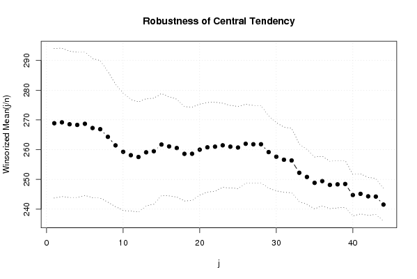
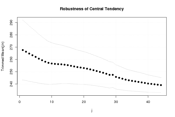
geomean <- function(x) { return(exp(mean(log(x)))) } harmean <- function(x) { return(1/mean(1/x)) } quamean <- function(x) { return(sqrt(mean(x*x))) } winmean <- function(x) { x <-sort(x[!is.na(x)]) n<-length(x) denom <- 3 nodenom <- n/denom if (nodenom>40) denom <- n/40 sqrtn = sqrt(n) roundnodenom = floor(nodenom) win <- array(NA,dim=c(roundnodenom,2)) for (j in 1:roundnodenom) { win[j,1] <- (j*x[j+1]+sum(x[(j+1):(n-j)])+j*x[n-j])/n win[j,2] <- sd(c(rep(x[j+1],j),x[(j+1):(n-j)],rep(x[n-j],j)))/sqrtn } return(win) } trimean <- function(x) { x <-sort(x[!is.na(x)]) n<-length(x) denom <- 3 nodenom <- n/denom if (nodenom>40) denom <- n/40 sqrtn = sqrt(n) roundnodenom = floor(nodenom) tri <- array(NA,dim=c(roundnodenom,2)) for (j in 1:roundnodenom) { tri[j,1] <- mean(x,trim=j/n) tri[j,2] <- sd(x[(j+1):(n-j)]) / sqrt(n-j*2) } return(tri) } midrange <- function(x) { return((max(x)+min(x))/2) } q1 <- function(data,n,p,i,f) { np <- n*p; i <<- floor(np) f <<- np - i qvalue <- (1-f)*data[i] + f*data[i+1] } q2 <- function(data,n,p,i,f) { np <- (n+1)*p i <<- floor(np) f <<- np - i qvalue <- (1-f)*data[i] + f*data[i+1] } q3 <- function(data,n,p,i,f) { np <- n*p i <<- floor(np) f <<- np - i if (f==0) { qvalue <- data[i] } else { qvalue <- data[i+1] } } q4 <- function(data,n,p,i,f) { np <- n*p i <<- floor(np) f <<- np - i if (f==0) { qvalue <- (data[i]+data[i+1])/2 } else { qvalue <- data[i+1] } } q5 <- function(data,n,p,i,f) { np <- (n-1)*p i <<- floor(np) f <<- np - i if (f==0) { qvalue <- data[i+1] } else { qvalue <- data[i+1] + f*(data[i+2]-data[i+1]) } } q6 <- function(data,n,p,i,f) { np <- n*p+0.5 i <<- floor(np) f <<- np - i qvalue <- data[i] } q7 <- function(data,n,p,i,f) { np <- (n+1)*p i <<- floor(np) f <<- np - i if (f==0) { qvalue <- data[i] } else { qvalue <- f*data[i] + (1-f)*data[i+1] } } q8 <- function(data,n,p,i,f) { np <- (n+1)*p i <<- floor(np) f <<- np - i if (f==0) { qvalue <- data[i] } else { if (f == 0.5) { qvalue <- (data[i]+data[i+1])/2 } else { if (f < 0.5) { qvalue <- data[i] } else { qvalue <- data[i+1] } } } } midmean <- function(x,def) { x <-sort(x[!is.na(x)]) n<-length(x) if (def==1) { qvalue1 <- q1(x,n,0.25,i,f) qvalue3 <- q1(x,n,0.75,i,f) } if (def==2) { qvalue1 <- q2(x,n,0.25,i,f) qvalue3 <- q2(x,n,0.75,i,f) } if (def==3) { qvalue1 <- q3(x,n,0.25,i,f) qvalue3 <- q3(x,n,0.75,i,f) } if (def==4) { qvalue1 <- q4(x,n,0.25,i,f) qvalue3 <- q4(x,n,0.75,i,f) } if (def==5) { qvalue1 <- q5(x,n,0.25,i,f) qvalue3 <- q5(x,n,0.75,i,f) } if (def==6) { qvalue1 <- q6(x,n,0.25,i,f) qvalue3 <- q6(x,n,0.75,i,f) } if (def==7) { qvalue1 <- q7(x,n,0.25,i,f) qvalue3 <- q7(x,n,0.75,i,f) } if (def==8) { qvalue1 <- q8(x,n,0.25,i,f) qvalue3 <- q8(x,n,0.75,i,f) } midm <- 0 myn <- 0 roundno4 <- round(n/4) round3no4 <- round(3*n/4) for (i in 1:n) { if ((x[i]>=qvalue1) & (x[i]<=qvalue3)){ midm = midm + x[i] myn = myn + 1 } } midm = midm / myn return(midm) } (arm <- mean(x)) sqrtn <- sqrt(length(x)) (armse <- sd(x) / sqrtn) (armose <- arm / armse) (geo <- geomean(x)) (har <- harmean(x)) (qua <- quamean(x)) (win <- winmean(x)) (tri <- trimean(x)) (midr <- midrange(x)) midm <- array(NA,dim=8) for (j in 1:8) midm[j] <- midmean(x,j) midm bitmap(file='test1.png') lb <- win[,1] - 2*win[,2] ub <- win[,1] + 2*win[,2] if ((ylimmin == '') | (ylimmax == '')) plot(win[,1],type='b',main=main, xlab='j', pch=19, ylab='Winsorized Mean(j/n)', ylim=c(min(lb),max(ub))) else plot(win[,1],type='l',main=main, xlab='j', pch=19, ylab='Winsorized Mean(j/n)', ylim=c(ylimmin,ylimmax)) lines(ub,lty=3) lines(lb,lty=3) grid() dev.off() bitmap(file='test2.png') lb <- tri[,1] - 2*tri[,2] ub <- tri[,1] + 2*tri[,2] if ((ylimmin == '') | (ylimmax == '')) plot(tri[,1],type='b',main=main, xlab='j', pch=19, ylab='Trimmed Mean(j/n)', ylim=c(min(lb),max(ub))) else plot(tri[,1],type='l',main=main, xlab='j', pch=19, ylab='Trimmed Mean(j/n)', ylim=c(ylimmin,ylimmax)) lines(ub,lty=3) lines(lb,lty=3) grid() dev.off() load(file='createtable') a<-table.start() a<-table.row.start(a) a<-table.element(a,'Central Tendency - Ungrouped Data',4,TRUE) a<-table.row.end(a) a<-table.row.start(a) a<-table.element(a,'Measure',header=TRUE) a<-table.element(a,'Value',header=TRUE) a<-table.element(a,'S.E.',header=TRUE) a<-table.element(a,'Value/S.E.',header=TRUE) a<-table.row.end(a) a<-table.row.start(a) a<-table.element(a,hyperlink('http://www.xycoon.com/arithmetic_mean.htm', 'Arithmetic Mean', 'click to view the definition of the Arithmetic Mean'),header=TRUE) a<-table.element(a,arm) a<-table.element(a,hyperlink('http://www.xycoon.com/arithmetic_mean_standard_error.htm', armse, 'click to view the definition of the Standard Error of the Arithmetic Mean')) a<-table.element(a,armose) a<-table.row.end(a) a<-table.row.start(a) a<-table.element(a,hyperlink('http://www.xycoon.com/geometric_mean.htm', 'Geometric Mean', 'click to view the definition of the Geometric Mean'),header=TRUE) a<-table.element(a,geo) a<-table.element(a,'') a<-table.element(a,'') a<-table.row.end(a) a<-table.row.start(a) a<-table.element(a,hyperlink('http://www.xycoon.com/harmonic_mean.htm', 'Harmonic Mean', 'click to view the definition of the Harmonic Mean'),header=TRUE) a<-table.element(a,har) a<-table.element(a,'') a<-table.element(a,'') a<-table.row.end(a) a<-table.row.start(a) a<-table.element(a,hyperlink('http://www.xycoon.com/quadratic_mean.htm', 'Quadratic Mean', 'click to view the definition of the Quadratic Mean'),header=TRUE) a<-table.element(a,qua) a<-table.element(a,'') a<-table.element(a,'') a<-table.row.end(a) for (j in 1:length(win[,1])) { a<-table.row.start(a) mylabel <- paste('Winsorized Mean (',j) mylabel <- paste(mylabel,'/') mylabel <- paste(mylabel,length(win[,1])) mylabel <- paste(mylabel,')') a<-table.element(a,hyperlink('http://www.xycoon.com/winsorized_mean.htm', mylabel, 'click to view the definition of the Winsorized Mean'),header=TRUE) a<-table.element(a,win[j,1]) a<-table.element(a,win[j,2]) a<-table.element(a,win[j,1]/win[j,2]) a<-table.row.end(a) } for (j in 1:length(tri[,1])) { a<-table.row.start(a) mylabel <- paste('Trimmed Mean (',j) mylabel <- paste(mylabel,'/') mylabel <- paste(mylabel,length(tri[,1])) mylabel <- paste(mylabel,')') a<-table.element(a,hyperlink('http://www.xycoon.com/arithmetic_mean.htm', mylabel, 'click to view the definition of the Trimmed Mean'),header=TRUE) a<-table.element(a,tri[j,1]) a<-table.element(a,tri[j,2]) a<-table.element(a,tri[j,1]/tri[j,2]) a<-table.row.end(a) } a<-table.row.start(a) a<-table.element(a,hyperlink('http://www.xycoon.com/median_1.htm', 'Median', 'click to view the definition of the Median'),header=TRUE) a<-table.element(a,median(x)) a<-table.element(a,'') a<-table.element(a,'') a<-table.row.end(a) a<-table.row.start(a) a<-table.element(a,hyperlink('http://www.xycoon.com/midrange.htm', 'Midrange', 'click to view the definition of the Midrange'),header=TRUE) a<-table.element(a,midr) a<-table.element(a,'') a<-table.element(a,'') a<-table.row.end(a) a<-table.row.start(a) mymid <- hyperlink('http://www.xycoon.com/midmean.htm', 'Midmean', 'click to view the definition of the Midmean') mylabel <- paste(mymid,hyperlink('http://www.xycoon.com/method_1.htm','Weighted Average at Xnp',''),sep=' - ') a<-table.element(a,mylabel,header=TRUE) a<-table.element(a,midm[1]) a<-table.element(a,'') a<-table.element(a,'') a<-table.row.end(a) a<-table.row.start(a) mymid <- hyperlink('http://www.xycoon.com/midmean.htm', 'Midmean', 'click to view the definition of the Midmean') mylabel <- paste(mymid,hyperlink('http://www.xycoon.com/method_2.htm','Weighted Average at X(n+1)p',''),sep=' - ') a<-table.element(a,mylabel,header=TRUE) a<-table.element(a,midm[2]) a<-table.element(a,'') a<-table.element(a,'') a<-table.row.end(a) a<-table.row.start(a) mymid <- hyperlink('http://www.xycoon.com/midmean.htm', 'Midmean', 'click to view the definition of the Midmean') mylabel <- paste(mymid,hyperlink('http://www.xycoon.com/method_3.htm','Empirical Distribution Function',''),sep=' - ') a<-table.element(a,mylabel,header=TRUE) a<-table.element(a,midm[3]) a<-table.element(a,'') a<-table.element(a,'') a<-table.row.end(a) a<-table.row.start(a) mymid <- hyperlink('http://www.xycoon.com/midmean.htm', 'Midmean', 'click to view the definition of the Midmean') mylabel <- paste(mymid,hyperlink('http://www.xycoon.com/method_4.htm','Empirical Distribution Function - Averaging',''),sep=' - ') a<-table.element(a,mylabel,header=TRUE) a<-table.element(a,midm[4]) a<-table.element(a,'') a<-table.element(a,'') a<-table.row.end(a) a<-table.row.start(a) mymid <- hyperlink('http://www.xycoon.com/midmean.htm', 'Midmean', 'click to view the definition of the Midmean') mylabel <- paste(mymid,hyperlink('http://www.xycoon.com/method_5.htm','Empirical Distribution Function - Interpolation',''),sep=' - ') a<-table.element(a,mylabel,header=TRUE) a<-table.element(a,midm[5]) a<-table.element(a,'') a<-table.element(a,'') a<-table.row.end(a) a<-table.row.start(a) mymid <- hyperlink('http://www.xycoon.com/midmean.htm', 'Midmean', 'click to view the definition of the Midmean') mylabel <- paste(mymid,hyperlink('http://www.xycoon.com/method_6.htm','Closest Observation',''),sep=' - ') a<-table.element(a,mylabel,header=TRUE) a<-table.element(a,midm[6]) a<-table.element(a,'') a<-table.element(a,'') a<-table.row.end(a) a<-table.row.start(a) mymid <- hyperlink('http://www.xycoon.com/midmean.htm', 'Midmean', 'click to view the definition of the Midmean') mylabel <- paste(mymid,hyperlink('http://www.xycoon.com/method_7.htm','True Basic - Statistics Graphics Toolkit',''),sep=' - ') a<-table.element(a,mylabel,header=TRUE) a<-table.element(a,midm[7]) a<-table.element(a,'') a<-table.element(a,'') a<-table.row.end(a) a<-table.row.start(a) mymid <- hyperlink('http://www.xycoon.com/midmean.htm', 'Midmean', 'click to view the definition of the Midmean') mylabel <- paste(mymid,hyperlink('http://www.xycoon.com/method_8.htm','MS Excel (old versions)',''),sep=' - ') a<-table.element(a,mylabel,header=TRUE) a<-table.element(a,midm[8]) a<-table.element(a,'') a<-table.element(a,'') a<-table.row.end(a) a<-table.row.start(a) a<-table.element(a,'Number of observations',header=TRUE) a<-table.element(a,length(x)) a<-table.element(a,'') a<-table.element(a,'') a<-table.row.end(a) a<-table.end(a) table.save(a,file='mytable.tab')

Copyright

This work is licensed under a Creative Commons Attribution-Noncommercial-Share Alike 3.0 License.

Software written by Ed van Stee & Patrick Wessa

Disclaimer

Information provided on this web site is provided "AS IS" without warranty of any kind, either express or implied, including, without limitation, warranties of merchantability, fitness for a particular purpose, and noninfringement. We use reasonable efforts to include accurate and timely information and periodically update the information, and software without notice. However, we make no warranties or representations as to the accuracy or completeness of such information (or software), and we assume no liability or responsibility for errors or omissions in the content of this web site, or any software bugs in online applications. Your use of this web site is AT YOUR OWN RISK. Under no circumstances and under no legal theory shall we be liable to you or any other person for any direct, indirect, special, incidental, exemplary, or consequential damages arising from your access to, or use of, this web site.

Privacy Policy

We may request personal information to be submitted to our servers in order to be able to:

• personalize online software applications according to your needs
• enforce strict security rules with respect to the data that you upload (e.g. statistical data)
• manage user sessions of online applications
• alert you about important changes or upgrades in resources or applications

We NEVER allow other companies to directly offer registered users information about their products and services. Banner references and hyperlinks of third parties NEVER contain any personal data of the visitor.

We do NOT sell, nor transmit by any means, personal information, nor statistical data series uploaded by you to third parties.

We carefully protect your data from loss, misuse, alteration, and destruction. However, at any time, and under any circumstance you are solely responsible for managing your passwords, and keeping them secret.

We store a unique ANONYMOUS USER ID in the form of a small 'Cookie' on your computer. This allows us to track your progress when using this website which is necessary to create state-dependent features. The cookie is used for NO OTHER PURPOSE. At any time you may opt to disallow cookies from this website - this will not affect other features of this website.

We examine cookies that are used by third-parties (banner and online ads) very closely: abuse from third-parties automatically results in termination of the advertising contract without refund. We have very good reason to believe that the cookies that are produced by third parties (banner ads) do NOT cause any privacy or security risk.

FreeStatistics.org is safe. There is no need to download any software to use the applications and services contained in this website. Hence, your system's security is not compromised by their use, and your personal data - other than data you submit in the account application form, and the user-agent information that is transmitted by your browser - is never transmitted to our servers.

As a general rule, we do not log on-line behavior of individuals (other than normal logging of webserver 'hits'). However, in cases of abuse, hacking, unauthorized access, Denial of Service attacks, illegal copying, hotlinking, non-compliance with international webstandards (such as robots.txt), or any other harmful behavior, our system engineers are empowered to log, track, identify, publish, and ban misbehaving individuals - even if this leads to ban entire blocks of IP addresses, or disclosing user's identity.

FreeStatistics.org is powered by