Free Statistics
of Irreproducible Research!
Description of Statistical Computation | |||||||||||||||||||||||||||||||||||||||||||||||||||||||||||||
|---|---|---|---|---|---|---|---|---|---|---|---|---|---|---|---|---|---|---|---|---|---|---|---|---|---|---|---|---|---|---|---|---|---|---|---|---|---|---|---|---|---|---|---|---|---|---|---|---|---|---|---|---|---|---|---|---|---|---|---|---|---|
| Author's title | |||||||||||||||||||||||||||||||||||||||||||||||||||||||||||||
| Author | *The author of this computation has been verified* | ||||||||||||||||||||||||||||||||||||||||||||||||||||||||||||
| R Software Module | rwasp_linear_regression.wasp | ||||||||||||||||||||||||||||||||||||||||||||||||||||||||||||
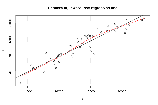
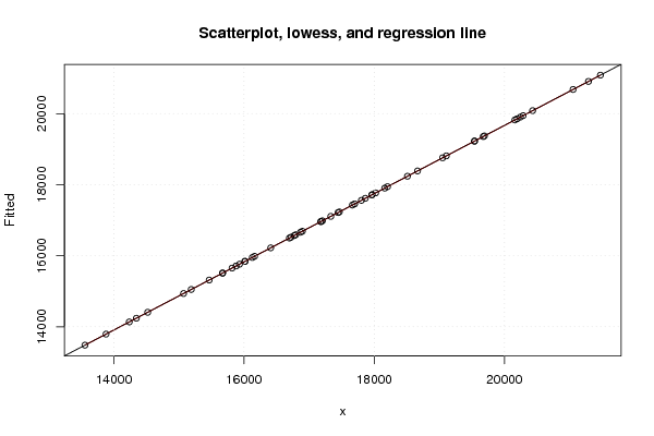
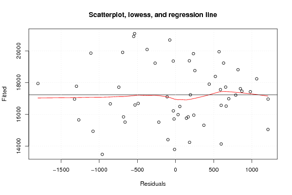
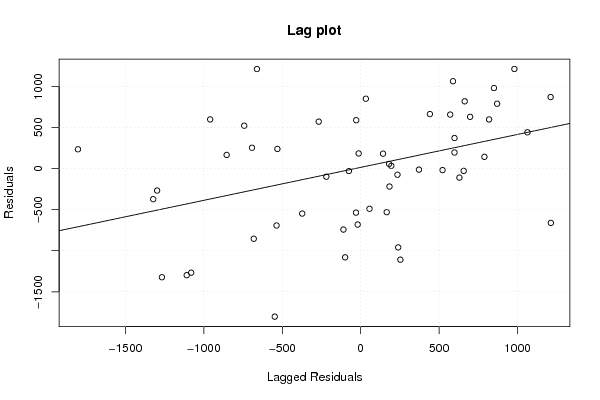
| Title produced by software | Linear Regression Graphical Model Validation | ||||||||||||||||||||||||||||||||||||||||||||||||||||||||||||
| Date of computation | Tue, 30 Nov 2010 09:48:39 +0000 | ||||||||||||||||||||||||||||||||||||||||||||||||||||||||||||
| Cite this page as follows | Statistical Computations at FreeStatistics.org, Office for Research Development and Education, URL https://freestatistics.org/blog/index.php?v=date/2010/Nov/30/t129111047651jgvk6a8eoa1nk.htm/, Retrieved Sat, 27 Apr 2024 10:20:58 +0000 | ||||||||||||||||||||||||||||||||||||||||||||||||||||||||||||
| Statistical Computations at FreeStatistics.org, Office for Research Development and Education, URL https://freestatistics.org/blog/index.php?pk=103267, Retrieved Sat, 27 Apr 2024 10:20:58 +0000 | |||||||||||||||||||||||||||||||||||||||||||||||||||||||||||||
| QR Codes: | |||||||||||||||||||||||||||||||||||||||||||||||||||||||||||||
|
| |||||||||||||||||||||||||||||||||||||||||||||||||||||||||||||
| Original text written by user: | |||||||||||||||||||||||||||||||||||||||||||||||||||||||||||||
| IsPrivate? | No (this computation is public) | ||||||||||||||||||||||||||||||||||||||||||||||||||||||||||||
| User-defined keywords | |||||||||||||||||||||||||||||||||||||||||||||||||||||||||||||
| Estimated Impact | 155 | ||||||||||||||||||||||||||||||||||||||||||||||||||||||||||||
Tree of Dependent Computations | |||||||||||||||||||||||||||||||||||||||||||||||||||||||||||||
| Family? (F = Feedback message, R = changed R code, M = changed R Module, P = changed Parameters, D = changed Data) | |||||||||||||||||||||||||||||||||||||||||||||||||||||||||||||
| - [Linear Regression Graphical Model Validation] [Colombia Coffee -...] [2008-02-26 10:22:06] [74be16979710d4c4e7c6647856088456] - M D [Linear Regression Graphical Model Validation] [Hypothese 1] [2010-11-11 10:31:04] [c1605865773cc027e55b238d879a644c] - [Linear Regression Graphical Model Validation] [Invoer en Uitvoer...] [2010-11-11 15:31:40] [62f7c80c4d96454bbd2b2b026ea9aad9] - D [Linear Regression Graphical Model Validation] [Invoer en Uitvoer...] [2010-11-11 15:38:29] [62f7c80c4d96454bbd2b2b026ea9aad9] - D [Linear Regression Graphical Model Validation] [Simple lineair re...] [2010-11-30 09:48:39] [8eb352cba3cf694c3df89d0a436a2f1b] [Current] | |||||||||||||||||||||||||||||||||||||||||||||||||||||||||||||
| Feedback Forum | |||||||||||||||||||||||||||||||||||||||||||||||||||||||||||||
Post a new message | |||||||||||||||||||||||||||||||||||||||||||||||||||||||||||||
Dataset | |||||||||||||||||||||||||||||||||||||||||||||||||||||||||||||
| Dataseries X: | |||||||||||||||||||||||||||||||||||||||||||||||||||||||||||||
16896.2 16698,00 19691.6 15930.7 17444.6 17699.4 15189.8 15672.7 17180.8 17664.9 17862.9 16162.3 17463.6 16772.1 19106.9 16721.3 18161.3 18509.9 17802.7 16409.9 17967.7 20286.6 19537.3 18021.9 20194.3 19049.6 20244.7 21473.3 19673.6 21053.2 20159.5 18203.6 21289.5 20432.3 17180.4 15816.8 15071.8 14521.1 15668.8 14346.9 13881,00 15465.9 14238.2 13557.7 16127.6 16793.9 16014,00 16867.9 16014.6 15878.6 18664.9 17962.5 17332.7 19542.1 17203.6 | |||||||||||||||||||||||||||||||||||||||||||||||||||||||||||||
| Dataseries Y: | |||||||||||||||||||||||||||||||||||||||||||||||||||||||||||||
16198.9 16554.2 19554.2 15903.8 18003.8 18329.6 16260.7 14851.9 18174.1 18406.6 18466.5 16016.5 17428.5 17167.2 19630,00 17183.6 18344.7 19301.4 18147.5 16192.9 18374.4 20515.2 18957.2 16471.5 18746.8 19009.5 19211.2 20547.7 19325.8 20605.5 20056.9 16141.4 20359.8 19711.6 15638.6 14384.5 13855.6 14308.3 15290.6 14423.8 13779.7 15686.3 14733.8 12522.5 16189.4 16059.1 16007.1 15806.8 15160,00 15692.1 18908.9 16969.9 16997.5 19858.9 17681.2 | |||||||||||||||||||||||||||||||||||||||||||||||||||||||||||||
Tables (Output of Computation) | |||||||||||||||||||||||||||||||||||||||||||||||||||||||||||||
| |||||||||||||||||||||||||||||||||||||||||||||||||||||||||||||
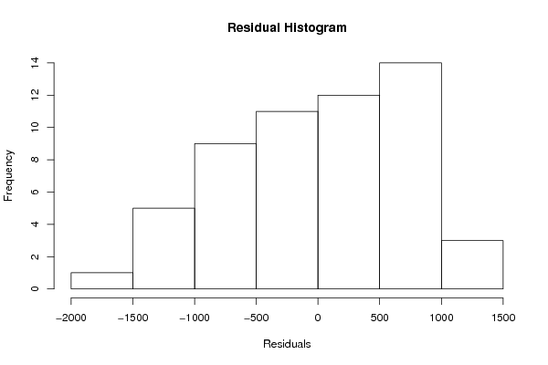
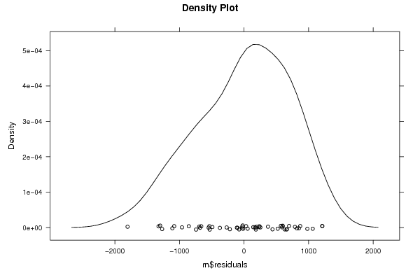
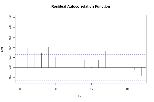
Figures (Output of Computation) | |||||||||||||||||||||||||||||||||||||||||||||||||||||||||||||
Input Parameters & R Code | |||||||||||||||||||||||||||||||||||||||||||||||||||||||||||||
| Parameters (Session): | |||||||||||||||||||||||||||||||||||||||||||||||||||||||||||||
| par1 = 0 ; | |||||||||||||||||||||||||||||||||||||||||||||||||||||||||||||
| Parameters (R input): | |||||||||||||||||||||||||||||||||||||||||||||||||||||||||||||
| par1 = 0 ; | |||||||||||||||||||||||||||||||||||||||||||||||||||||||||||||
| R code (references can be found in the software module): | |||||||||||||||||||||||||||||||||||||||||||||||||||||||||||||
par1 <- as.numeric(par1) | |||||||||||||||||||||||||||||||||||||||||||||||||||||||||||||