Free Statistics
of Irreproducible Research!
Description of Statistical Computation | |||||||||||||||||||||||||||||||||||||||||||||||||||||
|---|---|---|---|---|---|---|---|---|---|---|---|---|---|---|---|---|---|---|---|---|---|---|---|---|---|---|---|---|---|---|---|---|---|---|---|---|---|---|---|---|---|---|---|---|---|---|---|---|---|---|---|---|---|
| Author's title | |||||||||||||||||||||||||||||||||||||||||||||||||||||
| Author | *The author of this computation has been verified* | ||||||||||||||||||||||||||||||||||||||||||||||||||||
| R Software Module | rwasp_edauni.wasp | ||||||||||||||||||||||||||||||||||||||||||||||||||||
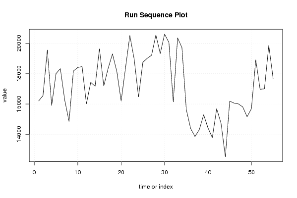
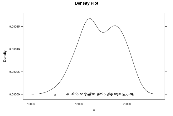
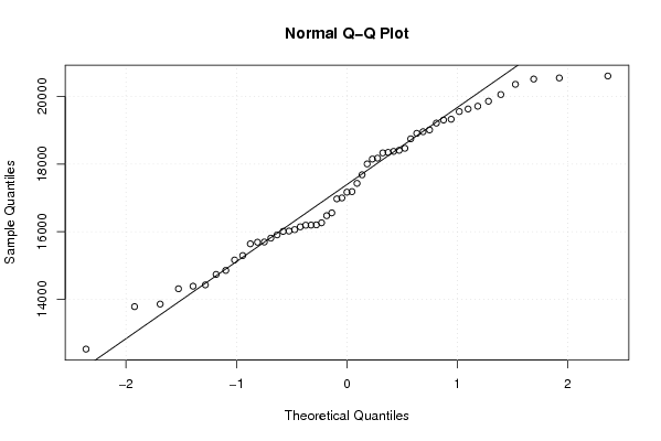
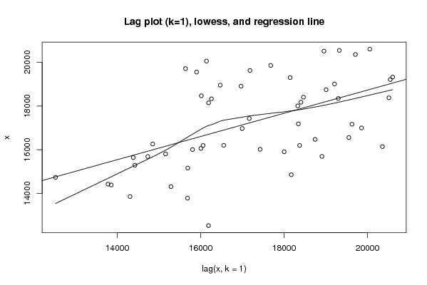
| Title produced by software | Univariate Explorative Data Analysis | ||||||||||||||||||||||||||||||||||||||||||||||||||||
| Date of computation | Fri, 26 Nov 2010 10:10:34 +0000 | ||||||||||||||||||||||||||||||||||||||||||||||||||||
| Cite this page as follows | Statistical Computations at FreeStatistics.org, Office for Research Development and Education, URL https://freestatistics.org/blog/index.php?v=date/2010/Nov/26/t12907663287g8x5q1w8vk7txb.htm/, Retrieved Sat, 06 Sep 2025 18:43:08 +0000 | ||||||||||||||||||||||||||||||||||||||||||||||||||||
| Statistical Computations at FreeStatistics.org, Office for Research Development and Education, URL https://freestatistics.org/blog/index.php?pk=101729, Retrieved Sat, 06 Sep 2025 18:43:08 +0000 | |||||||||||||||||||||||||||||||||||||||||||||||||||||
| QR Codes: | |||||||||||||||||||||||||||||||||||||||||||||||||||||
|
| |||||||||||||||||||||||||||||||||||||||||||||||||||||
| Original text written by user: | |||||||||||||||||||||||||||||||||||||||||||||||||||||
| IsPrivate? | No (this computation is public) | ||||||||||||||||||||||||||||||||||||||||||||||||||||
| User-defined keywords | |||||||||||||||||||||||||||||||||||||||||||||||||||||
| Estimated Impact | 269 | ||||||||||||||||||||||||||||||||||||||||||||||||||||
Tree of Dependent Computations | |||||||||||||||||||||||||||||||||||||||||||||||||||||
| Family? (F = Feedback message, R = changed R code, M = changed R Module, P = changed Parameters, D = changed Data) | |||||||||||||||||||||||||||||||||||||||||||||||||||||
| - [Univariate Explorative Data Analysis] [time effect in su...] [2010-11-17 08:55:33] [b98453cac15ba1066b407e146608df68] - D [Univariate Explorative Data Analysis] [Run sequence plot...] [2010-11-19 11:56:19] [2960375a246cc0628590c95c4038a43c] - D [Univariate Explorative Data Analysis] [Run Sequence Plot...] [2010-11-26 10:10:34] [4b5105369ca2b03f8f7589f5d63124c0] [Current] - D [Univariate Explorative Data Analysis] [Run Sequence Plot...] [2010-11-27 08:37:42] [62f7c80c4d96454bbd2b2b026ea9aad9] - D [Univariate Explorative Data Analysis] [Run Sequence Plot...] [2010-11-30 12:21:09] [d7a673bc47e3999e70f4e1e2276e5189] | |||||||||||||||||||||||||||||||||||||||||||||||||||||
| Feedback Forum | |||||||||||||||||||||||||||||||||||||||||||||||||||||
Post a new message | |||||||||||||||||||||||||||||||||||||||||||||||||||||
Dataset | |||||||||||||||||||||||||||||||||||||||||||||||||||||
| Dataseries X: | |||||||||||||||||||||||||||||||||||||||||||||||||||||
16198,9 16554,2 19554,2 15903,8 18003,8 18329,6 16260,7 14851,9 18174,1 18406,6 18466,5 16016,5 17428,5 17167,2 19630 17183,6 18344,7 19301,4 18147,5 16192,9 18374,4 20515,2 18957,2 16471,5 18746,8 19009,5 19211,2 20547,7 19325,8 20605,5 20056,9 16141,4 20359,8 19711,6 15638,6 14384,5 13855,6 14308,3 15290,6 14423,8 13779,7 15686,3 14733,8 12522,5 16189,4 16059,1 16007,1 15806,8 15160 15692,1 18908,9 16969,9 16997,5 19858,9 17681,2 | |||||||||||||||||||||||||||||||||||||||||||||||||||||
Tables (Output of Computation) | |||||||||||||||||||||||||||||||||||||||||||||||||||||
| |||||||||||||||||||||||||||||||||||||||||||||||||||||
Figures (Output of Computation) | |||||||||||||||||||||||||||||||||||||||||||||||||||||
Input Parameters & R Code | |||||||||||||||||||||||||||||||||||||||||||||||||||||
| Parameters (Session): | |||||||||||||||||||||||||||||||||||||||||||||||||||||
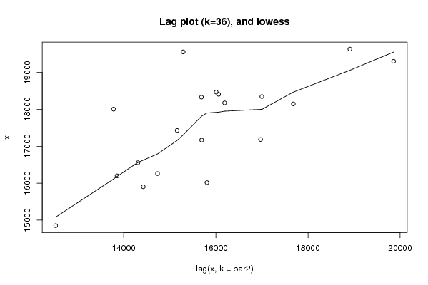
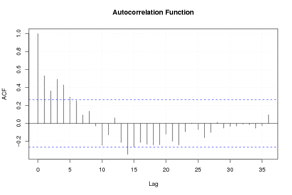
| par1 = 0 ; par2 = 36 ; | |||||||||||||||||||||||||||||||||||||||||||||||||||||
| Parameters (R input): | |||||||||||||||||||||||||||||||||||||||||||||||||||||
| par1 = 0 ; par2 = 36 ; | |||||||||||||||||||||||||||||||||||||||||||||||||||||
| R code (references can be found in the software module): | |||||||||||||||||||||||||||||||||||||||||||||||||||||
par1 <- as.numeric(par1) | |||||||||||||||||||||||||||||||||||||||||||||||||||||