Free Statistics
of Irreproducible Research!
Description of Statistical Computation | |||||||||||||||||||||||||||||||||||||||||||||||||||||||||||||
|---|---|---|---|---|---|---|---|---|---|---|---|---|---|---|---|---|---|---|---|---|---|---|---|---|---|---|---|---|---|---|---|---|---|---|---|---|---|---|---|---|---|---|---|---|---|---|---|---|---|---|---|---|---|---|---|---|---|---|---|---|---|
| Author's title | |||||||||||||||||||||||||||||||||||||||||||||||||||||||||||||
| Author | *The author of this computation has been verified* | ||||||||||||||||||||||||||||||||||||||||||||||||||||||||||||
| R Software Module | rwasp_linear_regression.wasp | ||||||||||||||||||||||||||||||||||||||||||||||||||||||||||||
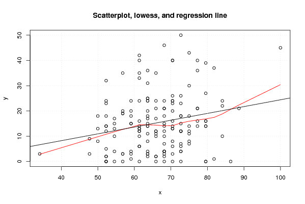
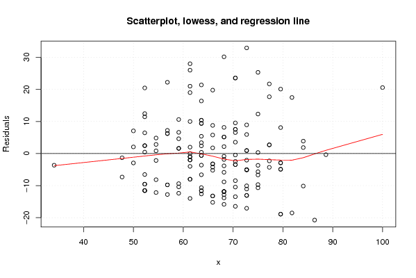
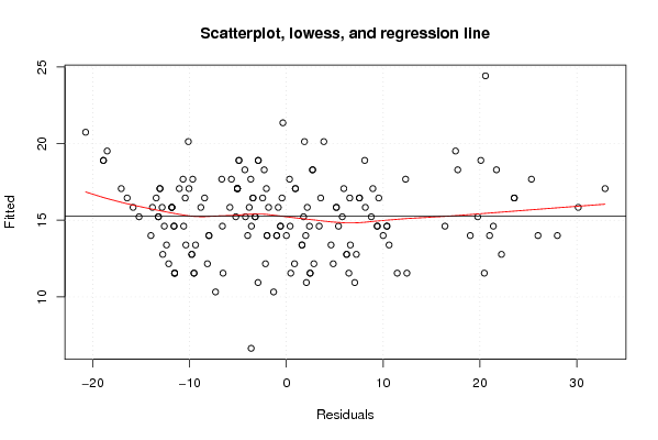
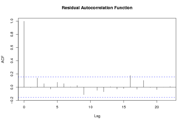
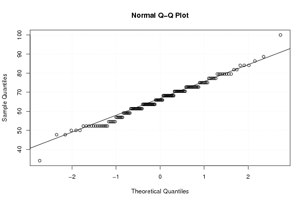
| Title produced by software | Linear Regression Graphical Model Validation | ||||||||||||||||||||||||||||||||||||||||||||||||||||||||||||
| Date of computation | Tue, 16 Nov 2010 09:49:54 +0000 | ||||||||||||||||||||||||||||||||||||||||||||||||||||||||||||
| Cite this page as follows | Statistical Computations at FreeStatistics.org, Office for Research Development and Education, URL https://freestatistics.org/blog/index.php?v=date/2010/Nov/16/t1289900967lj4euy374yyxso7.htm/, Retrieved Sat, 16 May 2026 11:21:10 +0000 | ||||||||||||||||||||||||||||||||||||||||||||||||||||||||||||
| Statistical Computations at FreeStatistics.org, Office for Research Development and Education, URL https://freestatistics.org/blog/index.php?pk=95304, Retrieved Sat, 16 May 2026 11:21:10 +0000 | |||||||||||||||||||||||||||||||||||||||||||||||||||||||||||||
| QR Codes: | |||||||||||||||||||||||||||||||||||||||||||||||||||||||||||||
|
| |||||||||||||||||||||||||||||||||||||||||||||||||||||||||||||
| Original text written by user: | |||||||||||||||||||||||||||||||||||||||||||||||||||||||||||||
| IsPrivate? | No (this computation is public) | ||||||||||||||||||||||||||||||||||||||||||||||||||||||||||||
| User-defined keywords | |||||||||||||||||||||||||||||||||||||||||||||||||||||||||||||
| Estimated Impact | 471 | ||||||||||||||||||||||||||||||||||||||||||||||||||||||||||||
Tree of Dependent Computations | |||||||||||||||||||||||||||||||||||||||||||||||||||||||||||||
| Family? (F = Feedback message, R = changed R code, M = changed R Module, P = changed Parameters, D = changed Data) | |||||||||||||||||||||||||||||||||||||||||||||||||||||||||||||
| - [Linear Regression Graphical Model Validation] [Colombia Coffee -...] [2008-02-26 10:22:06] [74be16979710d4c4e7c6647856088456] - M D [Linear Regression Graphical Model Validation] [ass 3 ws6] [2010-11-14 10:45:24] [0e7b3997dca5cf9d94982fb4db7bd3d5] - D [Linear Regression Graphical Model Validation] [mini tutorial] [2010-11-16 09:49:54] [3f56c8f677e988de577e4e00a8180a48] [Current] - D [Linear Regression Graphical Model Validation] [Huwelijken vs Tem...] [2010-12-18 13:15:27] [0e7b3997dca5cf9d94982fb4db7bd3d5] - D [Linear Regression Graphical Model Validation] [huwelijken vs bev...] [2010-12-18 13:19:35] [0e7b3997dca5cf9d94982fb4db7bd3d5] - D [Linear Regression Graphical Model Validation] [huwelijken vs wer...] [2010-12-18 13:22:08] [0e7b3997dca5cf9d94982fb4db7bd3d5] - D [Linear Regression Graphical Model Validation] [huwelijken vs wer...] [2010-12-18 15:55:05] [0e7b3997dca5cf9d94982fb4db7bd3d5] - D [Linear Regression Graphical Model Validation] [Huwelijken vs Tem...] [2010-12-18 15:56:52] [0e7b3997dca5cf9d94982fb4db7bd3d5] - D [Linear Regression Graphical Model Validation] [huwelijken vs bev...] [2010-12-18 15:59:42] [0e7b3997dca5cf9d94982fb4db7bd3d5] - RMPD [Kendall tau Correlation Matrix] [Pearson verband h...] [2010-12-18 17:25:13] [0e7b3997dca5cf9d94982fb4db7bd3d5] - RMPD [Kendall tau Correlation Matrix] [Pearson verband h...] [2010-12-18 17:29:57] [0e7b3997dca5cf9d94982fb4db7bd3d5] - RMPD [Kendall tau Correlation Matrix] [Kendall verband h...] [2010-12-18 17:30:57] [0e7b3997dca5cf9d94982fb4db7bd3d5] | |||||||||||||||||||||||||||||||||||||||||||||||||||||||||||||
| Feedback Forum | |||||||||||||||||||||||||||||||||||||||||||||||||||||||||||||
Post a new message | |||||||||||||||||||||||||||||||||||||||||||||||||||||||||||||
Dataset | |||||||||||||||||||||||||||||||||||||||||||||||||||||||||||||
| Dataseries X: | |||||||||||||||||||||||||||||||||||||||||||||||||||||||||||||
81,81818182 52,27272727 34,09090909 72,72727273 63,63636364 70,45454545 59,09090909 68,18181818 63,63636364 70,45454545 68,18181818 65,90909091 61,36363636 84,09090909 72,72727273 47,72727273 70,45454545 79,54545455 72,72727273 52,27272727 59,09090909 61,36363636 61,36363636 79,54545455 88,63636364 68,18181818 68,18181818 56,81818182 84,09090909 68,18181818 77,27272727 75 65,90909091 65,90909091 77,27272727 68,18181818 61,36363636 61,36363636 100 59,09090909 70,45454545 70,45454545 47,72727273 72,72727273 63,63636364 52,27272727 65,90909091 63,63636364 75 68,18181818 59,09090909 77,27272727 68,18181818 65,90909091 79,54545455 75 79,54545455 72,72727273 59,09090909 86,36363636 75 52,27272727 61,36363636 72,72727273 65,90909091 70,45454545 65,90909091 63,63636364 72,72727273 52,27272727 77,27272727 65,90909091 79,54545455 68,18181818 63,63636364 65,90909091 56,81818182 56,81818182 63,63636364 61,36363636 75 70,45454545 59,09090909 63,63636364 72,72727273 72,72727273 72,72727273 68,18181818 72,72727273 61,36363636 52,27272727 75 70,45454545 70,45454545 68,18181818 77,27272727 72,72727273 50 70,45454545 79,54545455 70,45454545 63,63636364 70,45454545 56,81818182 68,18181818 59,09090909 75 52,27272727 50 68,18181818 72,72727273 54,54545455 61,36363636 81,81818182 54,54545455 56,81818182 54,54545455 52,27272727 56,81818182 72,72727273 52,27272727 65,90909091 50 68,18181818 52,27272727 61,36363636 61,36363636 63,63636364 68,18181818 63,63636364 63,63636364 52,27272727 52,27272727 61,36363636 54,54545455 70,45454545 52,27272727 72,72727273 61,36363636 63,63636364 77,27272727 56,81818182 70,45454545 61,36363636 54,54545455 63,63636364 61,36363636 79,54545455 84,09090909 63,63636364 68,18181818 63,63636364 75 79,54545455 70,45454545 63,63636364 59,09090909 63,63636364 65,90909091 54,54545455 | |||||||||||||||||||||||||||||||||||||||||||||||||||||||||||||
| Dataseries Y: | |||||||||||||||||||||||||||||||||||||||||||||||||||||||||||||
37 2 3 6 17 14 3 4 18 40 0 35 12 22 50 3 3 16 12 2 4 16 6 0 21 21 2 35 10 4 36 7 17 10 14 7 12 14 45 15 20 16 9 26 15 12 12 11 30 14 24 16 10 2 14 11 16 4 15 0 12 0 13 18 11 13 24 20 12 14 21 21 0 46 2 0 3 3 25 13 18 24 20 24 23 15 7 3 0 35 14 8 0 13 12 21 12 18 6 39 8 25 26 19 4 18 14 18 13 21 4 15 0 1 0 0 10 24 19 12 0 2 8 24 23 42 6 24 18 3 14 0 32 10 4 23 5 18 24 36 40 20 40 33 17 14 40 27 24 4 15 8 43 14 24 3 1 31 12 13 | |||||||||||||||||||||||||||||||||||||||||||||||||||||||||||||
Tables (Output of Computation) | |||||||||||||||||||||||||||||||||||||||||||||||||||||||||||||
| |||||||||||||||||||||||||||||||||||||||||||||||||||||||||||||
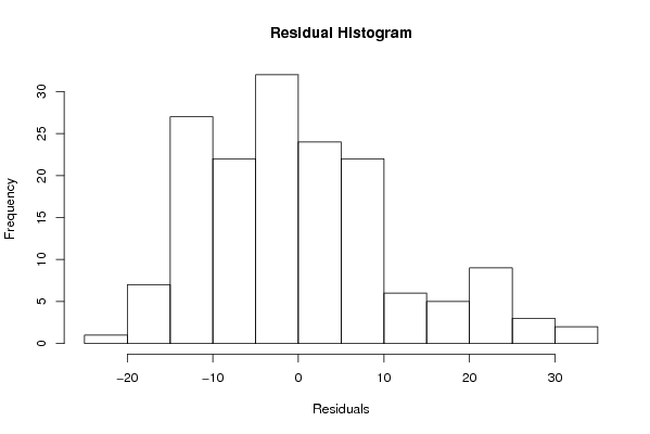
Figures (Output of Computation) | |||||||||||||||||||||||||||||||||||||||||||||||||||||||||||||
Input Parameters & R Code | |||||||||||||||||||||||||||||||||||||||||||||||||||||||||||||
| Parameters (Session): | |||||||||||||||||||||||||||||||||||||||||||||||||||||||||||||
| par1 = 0 ; | |||||||||||||||||||||||||||||||||||||||||||||||||||||||||||||
| Parameters (R input): | |||||||||||||||||||||||||||||||||||||||||||||||||||||||||||||
| par1 = 0 ; | |||||||||||||||||||||||||||||||||||||||||||||||||||||||||||||
| R code (references can be found in the software module): | |||||||||||||||||||||||||||||||||||||||||||||||||||||||||||||
par1 <- as.numeric(par1) | |||||||||||||||||||||||||||||||||||||||||||||||||||||||||||||