Free Statistics
of Irreproducible Research!
Description of Statistical Computation | |||||||||||||||||||||
|---|---|---|---|---|---|---|---|---|---|---|---|---|---|---|---|---|---|---|---|---|---|
| Author's title | |||||||||||||||||||||
| Author | *The author of this computation has been verified* | ||||||||||||||||||||
| R Software Module | rwasp_meanplot.wasp | ||||||||||||||||||||
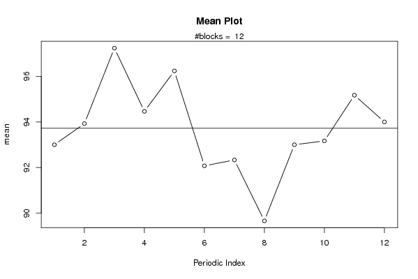
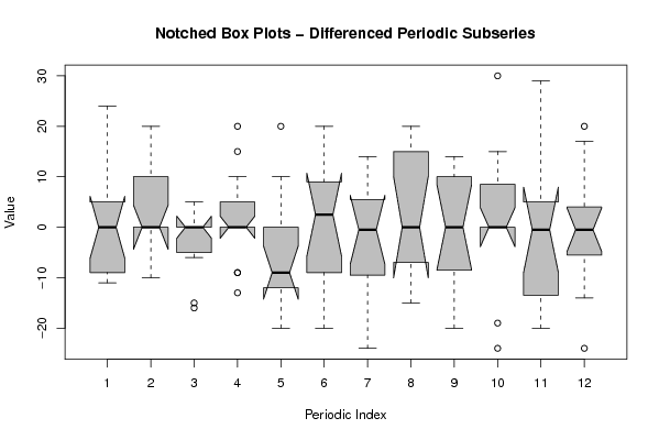
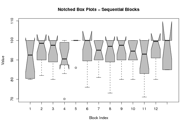
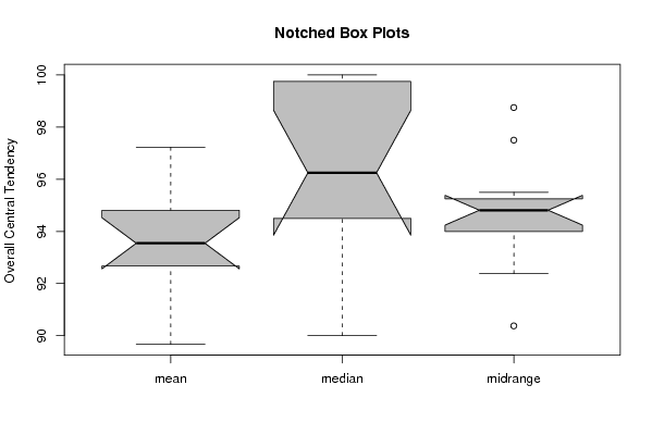
| Title produced by software | Mean Plot | ||||||||||||||||||||
| Date of computation | Fri, 12 Nov 2010 16:27:10 +0000 | ||||||||||||||||||||
| Cite this page as follows | Statistical Computations at FreeStatistics.org, Office for Research Development and Education, URL https://freestatistics.org/blog/index.php?v=date/2010/Nov/12/t1289579172qv3cmgyznvwoy8f.htm/, Retrieved Sun, 28 Apr 2024 05:02:07 +0000 | ||||||||||||||||||||
| Statistical Computations at FreeStatistics.org, Office for Research Development and Education, URL https://freestatistics.org/blog/index.php?pk=94231, Retrieved Sun, 28 Apr 2024 05:02:07 +0000 | |||||||||||||||||||||
| QR Codes: | |||||||||||||||||||||
|
| |||||||||||||||||||||
| Original text written by user: | |||||||||||||||||||||
| IsPrivate? | No (this computation is public) | ||||||||||||||||||||
| User-defined keywords | |||||||||||||||||||||
| Estimated Impact | 140 | ||||||||||||||||||||
Tree of Dependent Computations | |||||||||||||||||||||
| Family? (F = Feedback message, R = changed R code, M = changed R Module, P = changed Parameters, D = changed Data) | |||||||||||||||||||||
| - [Bivariate Data Series] [Bivariate dataset] [2008-01-05 23:51:08] [74be16979710d4c4e7c6647856088456] F RMPD [Mean Plot] [Colombia Coffee] [2008-01-07 13:38:24] [74be16979710d4c4e7c6647856088456] - RMPD [Mean Plot] [] [2010-11-12 16:27:10] [1d094c42a82a95b45a19e32ad4bfff5f] [Current] - D [Mean Plot] [] [2010-11-14 17:00:43] [d39e5c40c631ed6c22677d2e41dbfc7d] - D [Mean Plot] [] [2010-11-15 15:28:35] [d39e5c40c631ed6c22677d2e41dbfc7d] | |||||||||||||||||||||
| Feedback Forum | |||||||||||||||||||||
Post a new message | |||||||||||||||||||||
Dataset | |||||||||||||||||||||
| Dataseries X: | |||||||||||||||||||||
90 80 100 96 100 91 81 80 100 94 100 80 100 90 100 100 100 90 97 90 86 100 100 82 90 94 100 95 100 88 80 81 100 100 100 100 95 100 90 90 100 85 98 91 90 70 100 83 100 100 100 100 100 100 86 100 100 100 100 100 76 100 100 100 100 80 100 100 100 89 100 90 90 95 95 99 90 90 100 100 90 100 81 100 100 98 96 90 90 100 100 88 73 85 100 100 99 90 100 100 100 91 96 80 100 85 90 100 94 95 96 80 100 82 90 100 90 100 100 94 90 79 95 100 91 100 100 76 87 95 71 100 100 100 92 93 80 100 80 90 100 100 100 99 85 100 100 85 100 100 | |||||||||||||||||||||
Tables (Output of Computation) | |||||||||||||||||||||
| |||||||||||||||||||||
Figures (Output of Computation) | |||||||||||||||||||||
Input Parameters & R Code | |||||||||||||||||||||
| Parameters (Session): | |||||||||||||||||||||
| par1 = 12 ; | |||||||||||||||||||||
| Parameters (R input): | |||||||||||||||||||||
| par1 = 12 ; | |||||||||||||||||||||
| R code (references can be found in the software module): | |||||||||||||||||||||
par1 <- as.numeric(par1) | |||||||||||||||||||||