Free Statistics
of Irreproducible Research!
Description of Statistical Computation | |||||||||||||||||||||
|---|---|---|---|---|---|---|---|---|---|---|---|---|---|---|---|---|---|---|---|---|---|
| Author's title | |||||||||||||||||||||
| Author | *The author of this computation has been verified* | ||||||||||||||||||||
| R Software Module | rwasp_meanplot.wasp | ||||||||||||||||||||
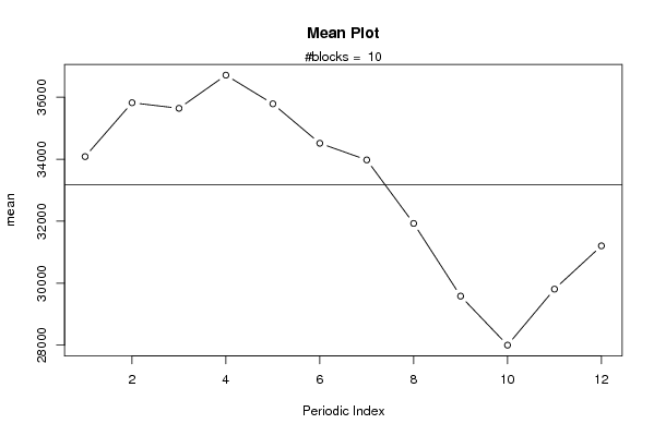
| Title produced by software | Mean Plot | ||||||||||||||||||||
| Date of computation | Fri, 12 Nov 2010 11:44:22 +0000 | ||||||||||||||||||||
| Cite this page as follows | Statistical Computations at FreeStatistics.org, Office for Research Development and Education, URL https://freestatistics.org/blog/index.php?v=date/2010/Nov/12/t1289562165jzo78z3qkha6l6u.htm/, Retrieved Tue, 16 Sep 2025 13:35:17 +0000 | ||||||||||||||||||||
| Statistical Computations at FreeStatistics.org, Office for Research Development and Education, URL https://freestatistics.org/blog/index.php?pk=94097, Retrieved Tue, 16 Sep 2025 13:35:17 +0000 | |||||||||||||||||||||
| QR Codes: | |||||||||||||||||||||
|
| |||||||||||||||||||||
| Original text written by user: | |||||||||||||||||||||
| IsPrivate? | No (this computation is public) | ||||||||||||||||||||
| User-defined keywords | |||||||||||||||||||||
| Estimated Impact | 284 | ||||||||||||||||||||
Tree of Dependent Computations | |||||||||||||||||||||
| Family? (F = Feedback message, R = changed R code, M = changed R Module, P = changed Parameters, D = changed Data) | |||||||||||||||||||||
| - [Bivariate Data Series] [Bivariate dataset] [2008-01-05 23:51:08] [74be16979710d4c4e7c6647856088456] F RMPD [Mean Plot] [Colombia Coffee] [2008-01-07 13:38:24] [74be16979710d4c4e7c6647856088456] - MPD [Mean Plot] [Retailprijs - Sei...] [2010-11-05 10:26:46] [aeb27d5c05332f2e597ad139ee63fbe4] - D [Mean Plot] [Mean Plot - VDAB ...] [2010-11-12 11:44:22] [18ef3d986e8801a4b28404e69e5bf56b] [Current] | |||||||||||||||||||||
| Feedback Forum | |||||||||||||||||||||
Post a new message | |||||||||||||||||||||
Dataset | |||||||||||||||||||||
| Dataseries X: | |||||||||||||||||||||
43880 43110 44496 44164 40399 36763 37903 35532 35533 32110 33374 35462 33508 36080 34560 38737 38144 37594 36424 36843 37246 38661 40454 44928 48441 48140 45998 47369 49554 47510 44873 45344 42413 36912 43452 42142 44382 43636 44167 44423 42868 43908 42013 38846 35087 33026 34646 37135 37985 43121 43722 43630 42234 39351 39327 35704 30466 28155 29257 29998 32529 34787 33855 34556 31348 30805 28353 24514 21106 21346 23335 24379 26290 30084 29429 30632 27349 27264 27474 24482 21453 18788 19282 19713 21917 23812 23785 24696 24562 23580 24939 23899 21454 19761 19815 20780 23462 25005 24725 26198 27543 26471 26558 25317 22896 22248 23406 25073 27691 30599 31948 32946 34012 32936 32974 30951 29812 29010 31068 32447 34844 35676 35387 36488 35652 33488 32914 29781 27951 | |||||||||||||||||||||
Tables (Output of Computation) | |||||||||||||||||||||
| |||||||||||||||||||||
Figures (Output of Computation) | |||||||||||||||||||||
Input Parameters & R Code | |||||||||||||||||||||
| Parameters (Session): | |||||||||||||||||||||
| par1 = 12 ; | |||||||||||||||||||||
| Parameters (R input): | |||||||||||||||||||||
| par1 = 12 ; | |||||||||||||||||||||
| R code (references can be found in the software module): | |||||||||||||||||||||
par1 <- as.numeric(par1) | |||||||||||||||||||||