*The author of this computation has been verified*

R Software Module: /rwasp_multipleregression.wasp (opens new window with default values)

Title produced by software: Multiple Regression

Date of computation: Fri, 24 Dec 2010 17:22:11 +0000

Cite this page as follows:

Statistical Computations at FreeStatistics.org, Office for Research Development and Education, URL http://www.freestatistics.org/blog/date/2010/Dec/24/t1293211610j9sdrog79td6b95.htm/, Retrieved Fri, 24 Dec 2010 18:27:01 +0100

BibTeX entries for LaTeX users:

@Manual{KEY, author = {{YOUR NAME}}, publisher = {Office for Research Development and Education}, title = {Statistical Computations at FreeStatistics.org, URL http://www.freestatistics.org/blog/date/2010/Dec/24/t1293211610j9sdrog79td6b95.htm/}, year = {2010}, } @Manual{R, title = {R: A Language and Environment for Statistical Computing}, author = {{R Development Core Team}}, organization = {R Foundation for Statistical Computing}, address = {Vienna, Austria}, year = {2010}, note = {{ISBN} 3-900051-07-0}, url = {http://www.R-project.org}, }

Original text written by user:

IsPrivate?

No (this computation is public)

User-defined keywords:

Dataseries X:

» Textbox « » Textfile « » CSV «

9506 1775 8704 2197 10079 2920 8993 4240 9957 5415 10240 6136 10098 6719 10090 6234 9867 7152 9736 3646 9040 2165 9232 2803 9520 1615 9217 2350 9868 3350 9455 3536 9984 5834 9556 6767 10190 5993 9906 7276 9824 5641 9972 3477 9185 2247 9765 2466 9838 1567 9084 2237 9643 2598 10051 3729 9987 5715 9827 5776 10491 5852 9722 6878 9472 5488 9728 3583 8510 2054 9511 2282 9492 1552 8638 2261 9792 2446 9605 3519 9237 5161 9533 5085 10293 5711 9938 6057 9984 5224 9563 3363 8871 1899 9301 2115 9215 1491 8834 2061 9998 2419 9604 3430 9507 4778 9718 4862 10095 6176 9583 5664 9883 5529 9365 3418 8919 1941 9449 2402 9769 1579 9321 2146 9939 2462 9336 3695 10195 4831 9464 5134 10010 6250 10213 5760 9563 6249 9890 2917 9305 1741 9391 2359 9743 1511 8587 2059 9731 2635 9563 2867 9998 4403 9437 5720 10038 4502 9918 5749 9252 5627 9737 2846 9035 1762 9133 2429 9487 1169 8700 2154 9627 2249 8947 2687 9283 4359 8829 5382 9947 4459 9628 6398 etc...

Output produced by software:

Enter (or paste) a matrix (table) containing all data (time) series. Every column represents a different variable and must be delimited by a space or Tab. Every row represents a period in time (or category) and must be delimited by hard returns. The easiest way to enter data is to copy and paste a block of spreadsheet cells. Please, do not use commas or spaces to seperate groups of digits! Summary of computational transaction Raw Input view raw input (R code) Raw Output view raw output of R engine Computing time 9 seconds R Server 'Gwilym Jenkins' @ 72.249.127.135 Multiple Linear Regression - Estimated Regression Equation births[t] = + 9490.9744697614 + 0.0169475520578264marriages[t] + 112.608867133597M1[t] -617.071094776177M2[t] + 299.958719086564M3[t] -56.3202608524251M4[t] + 112.035020095399M5[t] + 54.79846687321M6[t] + 596.171664979584M7[t] + 341.269535167487M8[t] + 157.120642050651M9[t] + 205.505306775077M10[t] -497.358074526631M11[t] + e[t] Multiple Linear Regression - Ordinary Least Squares Variable Parameter S.D. T-STAT H0: parameter = 0 2-tail p-value 1-tail p-value (Intercept) 9490.9744697614 164.836973 57.5779 0 0 marriages 0.0169475520578264 0.059211 0.2862 0.775205 0.387602 M1 112.608867133597 135.132206 0.8333 0.406332 0.203166 M2 -617.071094776177 126.504551 -4.8779 3e-06 2e-06 M3 299.958719086564 126.809947 2.3654 0.019626 0.009813 M4 -56.3202608524251 142.274214 -0.3959 0.692919 0.34646 M5 112.035020095399 200.305955 0.5593 0.576995 0.288497 M6 54.79846687321 222.076279 0.2468 0.805523 0.402761 M7 596.171664979584 231.812537 2.5718 0.011348 0.005674 M8 341.269535167487 257.068363 1.3275 0.18687 0.093435 M9 157.120642050651 226.395705 0.694 0.489029 0.244515 M10 205.505306775077 137.242705 1.4974 0.136941 0.06847 M11 -497.358074526631 128.196817 -3.8796 0.000172 8.6e-05 Multiple Linear Regression - Regression Statistics Multiple R 0.769552131893597 R-squared 0.59221048370198 Adjusted R-squared 0.551088851806381 F-TEST (value) 14.4014343887302 F-TEST (DF numerator) 12 F-TEST (DF denominator) 119 p-value 0 Multiple Linear Regression - Residual Statistics Residual Standard Deviation 296.084211333431 Sum Squared Residuals 10432237.3639118 Multiple Linear Regression - Actuals, Interpolation, and Residuals Time or Index Actuals Interpolation Forecast Residuals Prediction Error 1 9506 9633.66524179767 -127.665241797667 2 8704 8911.13714685626 -207.137146856263 3 10079 9840.42004085681 238.579959143186 4 8993 9506.51182963416 -513.511829634157 5 9957 9694.78048424993 262.219515750072 6 10240 9649.76311606143 590.23688393857 7 10098 10201.0167370175 -103.016737017518 8 10090 9937.89504445737 152.104955542625 9 9867 9769.30400412962 97.6959958703767 10 9736 9758.2705513393 -22.2705513393106 11 9040 9030.30784543996 9.69215456003966 12 9232 9538.47845817948 -306.478458179485 13 9520 9630.95363346839 -110.953633468384 14 9217 8913.73012232111 303.269877678888 15 9868 9847.70748824168 20.2925117583198 16 9455 9494.58075298545 -39.5807529854470 17 9984 9701.88150856216 282.118491437843 18 9556 9660.45702140992 -104.457021409920 19 10190 10188.7128142235 1.28718577646445 20 9906 9955.55439370163 -49.5543937016304 21 9824 9743.69625297025 80.3037470297523 22 9972 9755.40641504154 216.593584958462 23 9185 9031.6975447087 153.302455291298 24 9765 9532.767133136 232.232866864002 25 9838 9630.14015096961 207.859849030391 26 9084 8911.81504893858 172.184951061422 27 9643 9834.9629290942 -191.962929094195 28 10051 9497.8516305326 553.148369467393 29 9987 9699.86474986727 287.135250132725 30 9827 9643.66199732061 183.338002679387 31 10491 10186.3232093834 304.676790616618 32 9722 9948.80926798261 -226.809267982615 33 9472 9741.1032775054 -269.103277505400 34 9728 9757.20285555967 -29.2028555596671 35 8510 9028.42666716154 -518.426667161541 36 9511 9529.64878355736 -18.6487835573578 37 9492 9629.88593768874 -137.885937688742 38 8638 8912.22179018796 -274.221790187966 39 9792 9832.3869011814 -40.386901181405 40 9605 9494.29264460046 110.707355399536 41 9237 9690.47580602724 -453.475806027239 42 9533 9631.95123884865 -98.9512388486553 43 10293 10183.9336045432 109.066395456772 44 9938 9934.89532774314 3.10467225686013 45 9984 9736.62912376213 247.370876237866 46 9563 9753.47439410694 -190.474394106945 47 8871 9025.79979659258 -154.799796592579 48 9301 9526.8185423637 -225.818542363701 49 9215 9628.85213701321 -413.852137013215 50 8834 8908.8322797764 -74.8322797764004 51 9998 9831.92931727584 166.070682724156 52 9604 9492.78431246732 111.215687532683 53 9507 9683.9848935891 -176.984893589092 54 9718 9628.17193473976 89.82806526024 55 10095 10191.8142162501 -96.8142162501177 56 9583 9928.23493978441 -345.234939784414 57 9883 9741.79812713977 141.201872860229 58 9365 9754.40650947013 -389.406509470126 59 8919 9026.511593779 -107.511593779007 60 9449 9531.6824898043 -82.682489804297 61 9769 9630.3435215943 138.656478405697 62 9321 8910.27282170132 410.727178298684 63 9939 9832.65806201433 106.341937985670 64 9336 9497.27541376264 -161.275413762642 65 10195 9684.88311384816 510.116886151843 66 9464 9632.78166889949 -168.781668899489 67 10010 10193.0683351024 -183.068335102397 68 10213 9929.86190478196 283.138095218035 69 9563 9754.0003646214 -191.000364621406 70 9890 9745.91578588915 144.084214110845 71 9305 9023.12208336744 281.877916632558 72 9391 9530.9537450658 -139.953745065811 73 9743 9629.19108805437 113.808911945629 74 8587 8908.79838467229 -321.798384672285 75 9731 9835.58998852033 -104.589988520334 76 9563 9483.24284065876 79.757159341239 77 9998 9677.6295615674 320.370438432593 78 9437 9642.71293440538 -205.712934405375 79 10038 10163.4440141053 -125.444014105316 80 9918 9929.67548170933 -11.6754817093293 81 9252 9743.45898724144 -491.458987241438 82 9737 9744.71250969305 -7.71250969304891 83 9035 9023.47798196066 11.5220180393436 84 9133 9532.14007370986 -399.140073709858 85 9487 9623.3950252506 -136.395025250594 86 8700 8910.40840211778 -210.408402117778 87 9627 9829.04823342601 -202.048233426013 88 8947 9480.19228128835 -533.192281288352 89 9283 9676.88386927686 -393.883869276862 90 8829 9636.98466180983 -807.98466180983 91 9947 10162.7152693668 -215.715269366830 92 9628 9940.67444299486 -312.674442994859 93 9318 9725.98606106982 -407.986061069819 94 9605 9747.72917395934 -142.729173959342 95 8640 9025.59642596789 -385.596425967885 96 9214 9526.0559025211 -312.055902521099 97 9676 9626.47947972512 49.5205202748811 98 8642 8911.49304544948 -269.493045449479 99 9402 9832.64111446227 -430.641114462272 100 9610 9485.97139654007 124.028603459929 101 9294 9684.08657890144 -390.086578901439 102 9448 9630.0870081223 -182.087008122294 103 10319 10165.2235070714 153.776492928612 104 9548 9938.14925773824 -390.149257738243 105 9801 9729.59588965814 71.4041103418639 106 9596 9749.98319838303 -153.983198383033 107 8923 9025.98621966521 -102.986219665215 108 9746 9528.73361574624 217.266384253765 109 9829 9630.59773487517 198.402265124829 110 9125 8915.71298591188 209.287014088122 111 9782 9828.59064952045 -46.5906495204520 112 9441 9495.78402918155 -54.7840291815526 113 9162 9682.40877124771 -520.408771247714 114 9915 9629.86668994554 285.133310054457 115 10444 10184.9335101146 259.06648988536 116 10209 9925.11659020577 283.883409794226 117 9985 9732.83287210118 252.167127898819 118 9842 9751.18647457914 90.8135254208613 119 9429 9027.39286648601 401.607133513986 120 10132 9529.7504688697 602.249531130295 121 9849 9630.49604956282 218.503950437176 122 9172 8909.57797206695 262.422027933055 123 10313 9828.06527540666 484.934724593341 124 9819 9495.51286834863 323.487131651373 125 9955 9682.12066286273 272.879337137269 126 10048 9628.5617284371 419.43827156291 127 10082 10185.8147828216 -103.814782821647 128 10541 9927.13334890066 613.866651099344 129 10208 9738.59503980084 469.404960199158 130 10233 9748.7121319787 484.287868021304 131 9439 9027.680974871 411.319025129003 132 9963 9529.97078704646 433.029212953544 Goldfeld-Quandt test for Heteroskedasticity p-values Alternative Hypothesis breakpoint index greater 2-sided less 16 0.428469295891054 0.856938591782108 0.571530704108946 17 0.308047364164632 0.616094728329265 0.691952635835368 18 0.301746860802684 0.603493721605368 0.698253139197316 19 0.245131066918463 0.490262133836925 0.754868933081537 20 0.183815924959726 0.367631849919452 0.816184075040274 21 0.203624955362842 0.407249910725683 0.796375044637158 22 0.153090018936832 0.306180037873663 0.846909981063168 23 0.107458438249777 0.214916876499555 0.892541561750223 24 0.133776066622502 0.267552133245003 0.866223933377498 25 0.123489814132159 0.246979628264319 0.87651018586784 26 0.0872687370332102 0.174537474066420 0.91273126296679 27 0.114314707942611 0.228629415885223 0.885685292057389 28 0.365677033996537 0.731354067993075 0.634322966003463 29 0.312569778040793 0.625139556081585 0.687430221959207 30 0.272619669158251 0.545239338316503 0.727380330841749 31 0.250964463680516 0.501928927361032 0.749035536319484 32 0.219742208235716 0.439484416471431 0.780257791764284 33 0.274134923306819 0.548269846613637 0.725865076693181 34 0.222793911161626 0.445587822323252 0.777206088838374 35 0.341267579925405 0.68253515985081 0.658732420074595 36 0.280428437107616 0.560856874215232 0.719571562892384 37 0.235263559966969 0.470527119933938 0.764736440033031 38 0.239406208590949 0.478812417181897 0.760593791409051 39 0.195429884414929 0.390859768829859 0.80457011558507 40 0.156663615801206 0.313327231602412 0.843336384198794 41 0.313803821281608 0.627607642563217 0.686196178718391 42 0.297615340742852 0.595230681485705 0.702384659257148 43 0.250169801289801 0.500339602579602 0.749830198710199 44 0.203991535986623 0.407983071973246 0.796008464013377 45 0.188053034814978 0.376106069629956 0.811946965185022 46 0.166561592849768 0.333123185699535 0.833438407150232 47 0.135810625827595 0.27162125165519 0.864189374172405 48 0.118777396071408 0.237554792142815 0.881222603928592 49 0.137353313431134 0.274706626862268 0.862646686568866 50 0.108998546568528 0.217997093137055 0.891001453431472 51 0.0903563850370043 0.180712770074009 0.909643614962996 52 0.0710130560869455 0.142026112173891 0.928986943913054 53 0.0621764385295033 0.124352877059007 0.937823561470497 54 0.0475010256182521 0.0950020512365042 0.952498974381748 55 0.0372131289050968 0.0744262578101937 0.962786871094903 56 0.0386259612374103 0.0772519224748207 0.96137403876259 57 0.0302151806681549 0.0604303613363099 0.969784819331845 58 0.0352613316598047 0.0705226633196094 0.964738668340195 59 0.0266903118967951 0.0533806237935903 0.973309688103205 60 0.0194434129353150 0.0388868258706299 0.980556587064685 61 0.0160944645104593 0.0321889290209185 0.98390553548954 62 0.0221373225142798 0.0442746450285596 0.97786267748572 63 0.0164811631104850 0.0329623262209700 0.983518836889515 64 0.0128974879587655 0.0257949759175310 0.987102512041234 65 0.0257555274101711 0.0515110548203423 0.97424447258983 66 0.0221335163456032 0.0442670326912065 0.977866483654397 67 0.0176764521377542 0.0353529042755084 0.982323547862246 68 0.0181581904483262 0.0363163808966524 0.981841809551674 69 0.0146571963414812 0.0293143926829625 0.985342803658519 70 0.0114207434442114 0.0228414868884228 0.988579256555789 71 0.0116196206899549 0.0232392413799099 0.988380379310045 72 0.00874935460273151 0.0174987092054630 0.991250645397268 73 0.00644199379781378 0.0128839875956276 0.993558006202186 74 0.00697000337189522 0.0139400067437904 0.993029996628105 75 0.00495665028201107 0.00991330056402213 0.995043349717989 76 0.00334110647014846 0.00668221294029692 0.996658893529851 77 0.00382618181573984 0.00765236363147967 0.99617381818426 78 0.00307039926227455 0.00614079852454909 0.996929600737726 79 0.00225870507544064 0.00451741015088129 0.99774129492456 80 0.00145500201276848 0.00291000402553697 0.998544997987232 81 0.00295224765668204 0.00590449531336407 0.997047752343318 82 0.0019227109485727 0.0038454218971454 0.998077289051427 83 0.00123608075032111 0.00247216150064221 0.998763919249679 84 0.00203840871753650 0.00407681743507299 0.997961591282464 85 0.00151423321432551 0.00302846642865102 0.998485766785674 86 0.00120425725500039 0.00240851451000079 0.998795742745 87 0.0009113250341575 0.001822650068315 0.999088674965843 88 0.00269173800945986 0.00538347601891972 0.99730826199054 89 0.00313225132685393 0.00626450265370786 0.996867748673146 90 0.0291055808192445 0.058211161638489 0.970894419180756 91 0.0264317895046172 0.0528635790092344 0.973568210495383 92 0.0284729896982986 0.0569459793965972 0.971527010301701 93 0.0515794963929869 0.103158992785974 0.948420503607013 94 0.043911862838016 0.087823725676032 0.956088137161984 95 0.0720655619353627 0.144131123870725 0.927934438064637 96 0.151315151181419 0.302630302362838 0.848684848818581 97 0.126476171243944 0.252952342487888 0.873523828756056 98 0.154567625692103 0.309135251384205 0.845432374307897 99 0.225127137976169 0.450254275952338 0.774872862023831 100 0.187309458325151 0.374618916650302 0.812690541674849 101 0.178468491495112 0.356936982990223 0.821531508504888 102 0.214204192126755 0.428408384253509 0.785795807873245 103 0.207173218821966 0.414346437643931 0.792826781178034 104 0.397451886220607 0.794903772441215 0.602548113779393 105 0.346074333513492 0.692148667026984 0.653925666486508 106 0.382403948699787 0.764807897399574 0.617596051300213 107 0.465927178441299 0.931854356882598 0.534072821558701 108 0.461631939397953 0.923263878795907 0.538368060602047 109 0.376687879763607 0.753375759527213 0.623312120236393 110 0.294639972700540 0.589279945401079 0.70536002729946 111 0.350864484310401 0.701728968620802 0.649135515689599 112 0.335852380127941 0.671704760255882 0.66414761987206 113 0.75293024591123 0.494139508177542 0.247069754088771 114 0.66467933628295 0.6706413274341 0.33532066371705 115 0.692305482607014 0.615389034785972 0.307694517392986 116 0.664748671972499 0.670502656055002 0.335251328027501 Meta Analysis of Goldfeld-Quandt test for Heteroskedasticity Description # significant tests % significant tests OK/NOK 1% type I error level 15 0.148514851485149 NOK 5% type I error level 29 0.287128712871287 NOK 10% type I error level 40 0.396039603960396 NOK

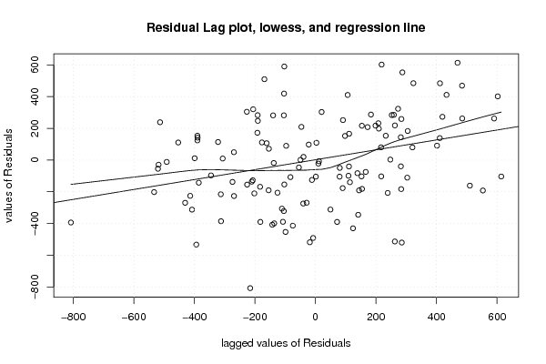
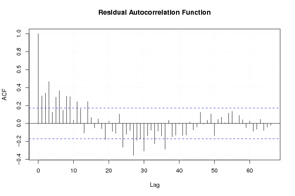
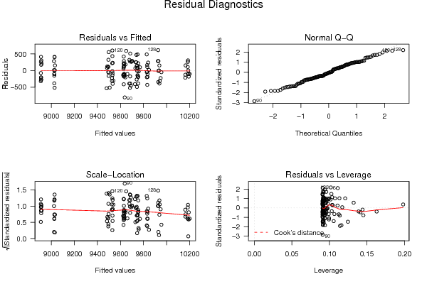
Charts produced by software:

http://www.freestatistics.org/blog/date/2010/Dec/24/t1293211610j9sdrog79td6b95/10o6j91293211321.png (open in new window) http://www.freestatistics.org/blog/date/2010/Dec/24/t1293211610j9sdrog79td6b95/10o6j91293211321.ps (open in new window) http://www.freestatistics.org/blog/date/2010/Dec/24/t1293211610j9sdrog79td6b95/1ckfr1293211321.png (open in new window) http://www.freestatistics.org/blog/date/2010/Dec/24/t1293211610j9sdrog79td6b95/1ckfr1293211321.ps (open in new window) http://www.freestatistics.org/blog/date/2010/Dec/24/t1293211610j9sdrog79td6b95/2ckfr1293211321.png (open in new window) http://www.freestatistics.org/blog/date/2010/Dec/24/t1293211610j9sdrog79td6b95/2ckfr1293211321.ps (open in new window) http://www.freestatistics.org/blog/date/2010/Dec/24/t1293211610j9sdrog79td6b95/35twc1293211321.png (open in new window) http://www.freestatistics.org/blog/date/2010/Dec/24/t1293211610j9sdrog79td6b95/35twc1293211321.ps (open in new window) http://www.freestatistics.org/blog/date/2010/Dec/24/t1293211610j9sdrog79td6b95/45twc1293211321.png (open in new window) http://www.freestatistics.org/blog/date/2010/Dec/24/t1293211610j9sdrog79td6b95/45twc1293211321.ps (open in new window) http://www.freestatistics.org/blog/date/2010/Dec/24/t1293211610j9sdrog79td6b95/55twc1293211321.png (open in new window) http://www.freestatistics.org/blog/date/2010/Dec/24/t1293211610j9sdrog79td6b95/55twc1293211321.ps (open in new window) http://www.freestatistics.org/blog/date/2010/Dec/24/t1293211610j9sdrog79td6b95/6xkdf1293211321.png (open in new window) http://www.freestatistics.org/blog/date/2010/Dec/24/t1293211610j9sdrog79td6b95/6xkdf1293211321.ps (open in new window) http://www.freestatistics.org/blog/date/2010/Dec/24/t1293211610j9sdrog79td6b95/78uci1293211321.png (open in new window) http://www.freestatistics.org/blog/date/2010/Dec/24/t1293211610j9sdrog79td6b95/78uci1293211321.ps (open in new window) http://www.freestatistics.org/blog/date/2010/Dec/24/t1293211610j9sdrog79td6b95/88uci1293211321.png (open in new window) http://www.freestatistics.org/blog/date/2010/Dec/24/t1293211610j9sdrog79td6b95/88uci1293211321.ps (open in new window) http://www.freestatistics.org/blog/date/2010/Dec/24/t1293211610j9sdrog79td6b95/98uci1293211321.png (open in new window) http://www.freestatistics.org/blog/date/2010/Dec/24/t1293211610j9sdrog79td6b95/98uci1293211321.ps (open in new window)

Parameters (Session):

par1 = 1 ; par2 = Include Monthly Dummies ; par3 = No Linear Trend ;

Parameters (R input):

par1 = 1 ; par2 = Include Monthly Dummies ; par3 = No Linear Trend ;

R code (references can be found in the software module):

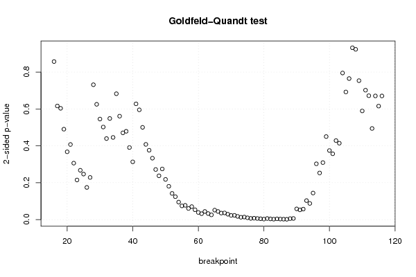
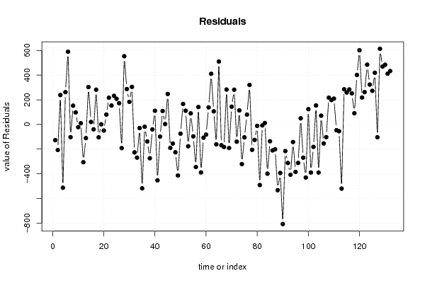
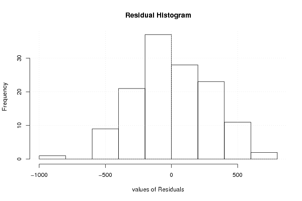
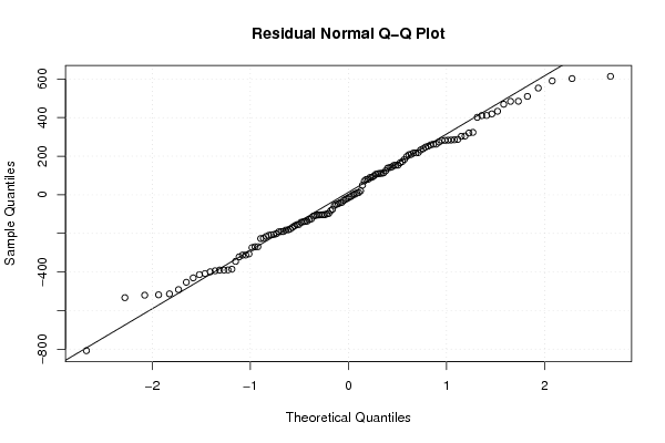
library(lattice) library(lmtest) n25 <- 25 #minimum number of obs. for Goldfeld-Quandt test par1 <- as.numeric(par1) x <- t(y) k <- length(x[1,]) n <- length(x[,1]) x1 <- cbind(x[,par1], x[,1:k!=par1]) mycolnames <- c(colnames(x)[par1], colnames(x)[1:k!=par1]) colnames(x1) <- mycolnames #colnames(x)[par1] x <- x1 if (par3 == 'First Differences'){ x2 <- array(0, dim=c(n-1,k), dimnames=list(1:(n-1), paste('(1-B)',colnames(x),sep=''))) for (i in 1:n-1) { for (j in 1:k) { x2[i,j] <- x[i+1,j] - x[i,j] } } x <- x2 } if (par2 == 'Include Monthly Dummies'){ x2 <- array(0, dim=c(n,11), dimnames=list(1:n, paste('M', seq(1:11), sep =''))) for (i in 1:11){ x2[seq(i,n,12),i] <- 1 } x <- cbind(x, x2) } if (par2 == 'Include Quarterly Dummies'){ x2 <- array(0, dim=c(n,3), dimnames=list(1:n, paste('Q', seq(1:3), sep =''))) for (i in 1:3){ x2[seq(i,n,4),i] <- 1 } x <- cbind(x, x2) } k <- length(x[1,]) if (par3 == 'Linear Trend'){ x <- cbind(x, c(1:n)) colnames(x)[k+1] <- 't' } x k <- length(x[1,]) df <- as.data.frame(x) (mylm <- lm(df)) (mysum <- summary(mylm)) if (n > n25) { kp3 <- k + 3 nmkm3 <- n - k - 3 gqarr <- array(NA, dim=c(nmkm3-kp3+1,3)) numgqtests <- 0 numsignificant1 <- 0 numsignificant5 <- 0 numsignificant10 <- 0 for (mypoint in kp3:nmkm3) { j <- 0 numgqtests <- numgqtests + 1 for (myalt in c('greater', 'two.sided', 'less')) { j <- j + 1 gqarr[mypoint-kp3+1,j] <- gqtest(mylm, point=mypoint, alternative=myalt)$p.value } if (gqarr[mypoint-kp3+1,2] < 0.01) numsignificant1 <- numsignificant1 + 1 if (gqarr[mypoint-kp3+1,2] < 0.05) numsignificant5 <- numsignificant5 + 1 if (gqarr[mypoint-kp3+1,2] < 0.10) numsignificant10 <- numsignificant10 + 1 } gqarr } bitmap(file='test0.png') plot(x[,1], type='l', main='Actuals and Interpolation', ylab='value of Actuals and Interpolation (dots)', xlab='time or index') points(x[,1]-mysum$resid) grid() dev.off() bitmap(file='test1.png') plot(mysum$resid, type='b', pch=19, main='Residuals', ylab='value of Residuals', xlab='time or index') grid() dev.off() bitmap(file='test2.png') hist(mysum$resid, main='Residual Histogram', xlab='values of Residuals') grid() dev.off() bitmap(file='test3.png') densityplot(~mysum$resid,col='black',main='Residual Density Plot', xlab='values of Residuals') dev.off() bitmap(file='test4.png') qqnorm(mysum$resid, main='Residual Normal Q-Q Plot') qqline(mysum$resid) grid() dev.off() (myerror <- as.ts(mysum$resid)) bitmap(file='test5.png') dum <- cbind(lag(myerror,k=1),myerror) dum dum1 <- dum[2:length(myerror),] dum1 z <- as.data.frame(dum1) z plot(z,main=paste('Residual Lag plot, lowess, and regression line'), ylab='values of Residuals', xlab='lagged values of Residuals') lines(lowess(z)) abline(lm(z)) grid() dev.off() bitmap(file='test6.png') acf(mysum$resid, lag.max=length(mysum$resid)/2, main='Residual Autocorrelation Function') grid() dev.off() bitmap(file='test7.png') pacf(mysum$resid, lag.max=length(mysum$resid)/2, main='Residual Partial Autocorrelation Function') grid() dev.off() bitmap(file='test8.png') opar <- par(mfrow = c(2,2), oma = c(0, 0, 1.1, 0)) plot(mylm, las = 1, sub='Residual Diagnostics') par(opar) dev.off() if (n > n25) { bitmap(file='test9.png') plot(kp3:nmkm3,gqarr[,2], main='Goldfeld-Quandt test',ylab='2-sided p-value',xlab='breakpoint') grid() dev.off() } load(file='createtable') a<-table.start() a<-table.row.start(a) a<-table.element(a, 'Multiple Linear Regression - Estimated Regression Equation', 1, TRUE) a<-table.row.end(a) myeq <- colnames(x)[1] myeq <- paste(myeq, '[t] = ', sep='') for (i in 1:k){ if (mysum$coefficients[i,1] > 0) myeq <- paste(myeq, '+', '') myeq <- paste(myeq, mysum$coefficients[i,1], sep=' ') if (rownames(mysum$coefficients)[i] != '(Intercept)') { myeq <- paste(myeq, rownames(mysum$coefficients)[i], sep='') if (rownames(mysum$coefficients)[i] != 't') myeq <- paste(myeq, '[t]', sep='') } } myeq <- paste(myeq, ' + e[t]') a<-table.row.start(a) a<-table.element(a, myeq) a<-table.row.end(a) a<-table.end(a) table.save(a,file='mytable1.tab') a<-table.start() a<-table.row.start(a) a<-table.element(a,hyperlink('http://www.xycoon.com/ols1.htm','Multiple Linear Regression - Ordinary Least Squares',''), 6, TRUE) a<-table.row.end(a) a<-table.row.start(a) a<-table.element(a,'Variable',header=TRUE) a<-table.element(a,'Parameter',header=TRUE) a<-table.element(a,'S.D.',header=TRUE) a<-table.element(a,'T-STAT<br />H0: parameter = 0',header=TRUE) a<-table.element(a,'2-tail p-value',header=TRUE) a<-table.element(a,'1-tail p-value',header=TRUE) a<-table.row.end(a) for (i in 1:k){ a<-table.row.start(a) a<-table.element(a,rownames(mysum$coefficients)[i],header=TRUE) a<-table.element(a,mysum$coefficients[i,1]) a<-table.element(a, round(mysum$coefficients[i,2],6)) a<-table.element(a, round(mysum$coefficients[i,3],4)) a<-table.element(a, round(mysum$coefficients[i,4],6)) a<-table.element(a, round(mysum$coefficients[i,4]/2,6)) a<-table.row.end(a) } a<-table.end(a) table.save(a,file='mytable2.tab') a<-table.start() a<-table.row.start(a) a<-table.element(a, 'Multiple Linear Regression - Regression Statistics', 2, TRUE) a<-table.row.end(a) a<-table.row.start(a) a<-table.element(a, 'Multiple R',1,TRUE) a<-table.element(a, sqrt(mysum$r.squared)) a<-table.row.end(a) a<-table.row.start(a) a<-table.element(a, 'R-squared',1,TRUE) a<-table.element(a, mysum$r.squared) a<-table.row.end(a) a<-table.row.start(a) a<-table.element(a, 'Adjusted R-squared',1,TRUE) a<-table.element(a, mysum$adj.r.squared) a<-table.row.end(a) a<-table.row.start(a) a<-table.element(a, 'F-TEST (value)',1,TRUE) a<-table.element(a, mysum$fstatistic[1]) a<-table.row.end(a) a<-table.row.start(a) a<-table.element(a, 'F-TEST (DF numerator)',1,TRUE) a<-table.element(a, mysum$fstatistic[2]) a<-table.row.end(a) a<-table.row.start(a) a<-table.element(a, 'F-TEST (DF denominator)',1,TRUE) a<-table.element(a, mysum$fstatistic[3]) a<-table.row.end(a) a<-table.row.start(a) a<-table.element(a, 'p-value',1,TRUE) a<-table.element(a, 1-pf(mysum$fstatistic[1],mysum$fstatistic[2],mysum$fstatistic[3])) a<-table.row.end(a) a<-table.row.start(a) a<-table.element(a, 'Multiple Linear Regression - Residual Statistics', 2, TRUE) a<-table.row.end(a) a<-table.row.start(a) a<-table.element(a, 'Residual Standard Deviation',1,TRUE) a<-table.element(a, mysum$sigma) a<-table.row.end(a) a<-table.row.start(a) a<-table.element(a, 'Sum Squared Residuals',1,TRUE) a<-table.element(a, sum(myerror*myerror)) a<-table.row.end(a) a<-table.end(a) table.save(a,file='mytable3.tab') a<-table.start() a<-table.row.start(a) a<-table.element(a, 'Multiple Linear Regression - Actuals, Interpolation, and Residuals', 4, TRUE) a<-table.row.end(a) a<-table.row.start(a) a<-table.element(a, 'Time or Index', 1, TRUE) a<-table.element(a, 'Actuals', 1, TRUE) a<-table.element(a, 'Interpolation<br />Forecast', 1, TRUE) a<-table.element(a, 'Residuals<br />Prediction Error', 1, TRUE) a<-table.row.end(a) for (i in 1:n) { a<-table.row.start(a) a<-table.element(a,i, 1, TRUE) a<-table.element(a,x[i]) a<-table.element(a,x[i]-mysum$resid[i]) a<-table.element(a,mysum$resid[i]) a<-table.row.end(a) } a<-table.end(a) table.save(a,file='mytable4.tab') if (n > n25) { a<-table.start() a<-table.row.start(a) a<-table.element(a,'Goldfeld-Quandt test for Heteroskedasticity',4,TRUE) a<-table.row.end(a) a<-table.row.start(a) a<-table.element(a,'p-values',header=TRUE) a<-table.element(a,'Alternative Hypothesis',3,header=TRUE) a<-table.row.end(a) a<-table.row.start(a) a<-table.element(a,'breakpoint index',header=TRUE) a<-table.element(a,'greater',header=TRUE) a<-table.element(a,'2-sided',header=TRUE) a<-table.element(a,'less',header=TRUE) a<-table.row.end(a) for (mypoint in kp3:nmkm3) { a<-table.row.start(a) a<-table.element(a,mypoint,header=TRUE) a<-table.element(a,gqarr[mypoint-kp3+1,1]) a<-table.element(a,gqarr[mypoint-kp3+1,2]) a<-table.element(a,gqarr[mypoint-kp3+1,3]) a<-table.row.end(a) } a<-table.end(a) table.save(a,file='mytable5.tab') a<-table.start() a<-table.row.start(a) a<-table.element(a,'Meta Analysis of Goldfeld-Quandt test for Heteroskedasticity',4,TRUE) a<-table.row.end(a) a<-table.row.start(a) a<-table.element(a,'Description',header=TRUE) a<-table.element(a,'# significant tests',header=TRUE) a<-table.element(a,'% significant tests',header=TRUE) a<-table.element(a,'OK/NOK',header=TRUE) a<-table.row.end(a) a<-table.row.start(a) a<-table.element(a,'1% type I error level',header=TRUE) a<-table.element(a,numsignificant1) a<-table.element(a,numsignificant1/numgqtests) if (numsignificant1/numgqtests < 0.01) dum <- 'OK' else dum <- 'NOK' a<-table.element(a,dum) a<-table.row.end(a) a<-table.row.start(a) a<-table.element(a,'5% type I error level',header=TRUE) a<-table.element(a,numsignificant5) a<-table.element(a,numsignificant5/numgqtests) if (numsignificant5/numgqtests < 0.05) dum <- 'OK' else dum <- 'NOK' a<-table.element(a,dum) a<-table.row.end(a) a<-table.row.start(a) a<-table.element(a,'10% type I error level',header=TRUE) a<-table.element(a,numsignificant10) a<-table.element(a,numsignificant10/numgqtests) if (numsignificant10/numgqtests < 0.1) dum <- 'OK' else dum <- 'NOK' a<-table.element(a,dum) a<-table.row.end(a) a<-table.end(a) table.save(a,file='mytable6.tab') }

Copyright

This work is licensed under a Creative Commons Attribution-Noncommercial-Share Alike 3.0 License.

Software written by Ed van Stee & Patrick Wessa

Disclaimer

Information provided on this web site is provided "AS IS" without warranty of any kind, either express or implied, including, without limitation, warranties of merchantability, fitness for a particular purpose, and noninfringement. We use reasonable efforts to include accurate and timely information and periodically update the information, and software without notice. However, we make no warranties or representations as to the accuracy or completeness of such information (or software), and we assume no liability or responsibility for errors or omissions in the content of this web site, or any software bugs in online applications. Your use of this web site is AT YOUR OWN RISK. Under no circumstances and under no legal theory shall we be liable to you or any other person for any direct, indirect, special, incidental, exemplary, or consequential damages arising from your access to, or use of, this web site.

Privacy Policy

We may request personal information to be submitted to our servers in order to be able to:

• personalize online software applications according to your needs
• enforce strict security rules with respect to the data that you upload (e.g. statistical data)
• manage user sessions of online applications
• alert you about important changes or upgrades in resources or applications

We NEVER allow other companies to directly offer registered users information about their products and services. Banner references and hyperlinks of third parties NEVER contain any personal data of the visitor.

We do NOT sell, nor transmit by any means, personal information, nor statistical data series uploaded by you to third parties.

We carefully protect your data from loss, misuse, alteration, and destruction. However, at any time, and under any circumstance you are solely responsible for managing your passwords, and keeping them secret.

We store a unique ANONYMOUS USER ID in the form of a small 'Cookie' on your computer. This allows us to track your progress when using this website which is necessary to create state-dependent features. The cookie is used for NO OTHER PURPOSE. At any time you may opt to disallow cookies from this website - this will not affect other features of this website.

We examine cookies that are used by third-parties (banner and online ads) very closely: abuse from third-parties automatically results in termination of the advertising contract without refund. We have very good reason to believe that the cookies that are produced by third parties (banner ads) do NOT cause any privacy or security risk.

FreeStatistics.org is safe. There is no need to download any software to use the applications and services contained in this website. Hence, your system's security is not compromised by their use, and your personal data - other than data you submit in the account application form, and the user-agent information that is transmitted by your browser - is never transmitted to our servers.

As a general rule, we do not log on-line behavior of individuals (other than normal logging of webserver 'hits'). However, in cases of abuse, hacking, unauthorized access, Denial of Service attacks, illegal copying, hotlinking, non-compliance with international webstandards (such as robots.txt), or any other harmful behavior, our system engineers are empowered to log, track, identify, publish, and ban misbehaving individuals - even if this leads to ban entire blocks of IP addresses, or disclosing user's identity.

FreeStatistics.org is powered by