Repository of Reproducible Computations

Free Statistics

of Irreproducible Research!

Author's title

Author

*The author of this computation has been verified*

R Software Module

rwasp_autocorrelation.wasp

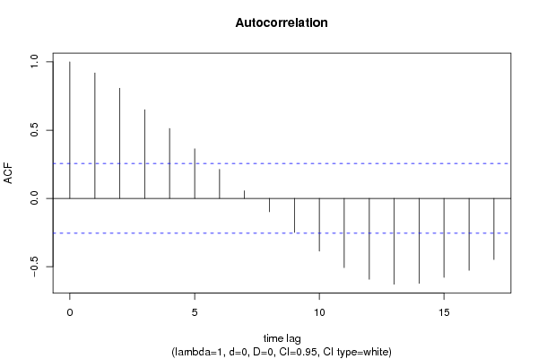
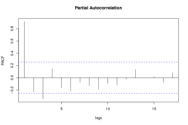
Title produced by software

(Partial) Autocorrelation Function

Date of computation

Tue, 21 Dec 2010 19:50:45 +0000

Cite this page as follows

Statistical Computations at FreeStatistics.org, Office for Research Development and Education, URL https://freestatistics.org/blog/index.php?v=date/2010/Dec/21/t1292960915mwag0oej257wtxp.htm/, Retrieved Thu, 09 May 2024 18:42:17 +0000

Statistical Computations at FreeStatistics.org, Office for Research Development and Education, URL https://freestatistics.org/blog/index.php?pk=113909, Retrieved Thu, 09 May 2024 18:42:17 +0000

QR Codes:

Paste this QR Code to cite your computation.

Original text written by user:

IsPrivate?

No (this computation is public)

User-defined keywords

Estimated Impact

130

Family? (F = Feedback message, R = changed R code, M = changed R Module, P = changed Parameters, D = changed Data)

-     [Univariate Data Series] [data set] [2008-12-01 19:54:57] [b98453cac15ba1066b407e146608df68]
- RMP   [(Partial) Autocorrelation Function] [Unemployment] [2010-11-29 09:05:21] [b98453cac15ba1066b407e146608df68]
-    D    [(Partial) Autocorrelation Function] [W9 ACF origineel] [2010-12-03 11:36:39] [56d90b683fcd93137645f9226b43c62b]
-   P       [(Partial) Autocorrelation Function] [Autocorrelatiefun...] [2010-12-07 20:51:20] [608064602fec1c42028cf50c6f981c88]
-   P         [(Partial) Autocorrelation Function] [AF zonder lags] [2010-12-07 21:06:36] [608064602fec1c42028cf50c6f981c88]
-   PD            [(Partial) Autocorrelation Function] [Autocorrelatiefun...] [2010-12-21 19:50:45] [8bf9de033bd61652831a8b7489bc3566] [Current]

Feedback Forum

Post a new message

Dataseries X:

Download CSV

Histogram

Boxplots

8.1
9.9
11.5
23.4
25.4
27.9
26.1
18.8
14.1
11.5
15.8
12.4
4.5
-2.2
-4.2
-9.4
-14.5
-17.9
-15.1
-15.2
-15.7
-18
-18.1
-13.5
-9.9
-4.8
-1.7
-0.1
2.2
10.2
7.6
10.8
3.8
11
10.8
20.1
14.9
13
10.9
9.6
4
-1.1
-7.7
-8.9
-8
-7.1
-5.3
-2.5
-2.4
-2.9
-4.8
-7.2
1.7
2.2
13.4
12.3
13.7
4.4
-2.5

Summary of computational transaction
Raw Input	view raw input (R code)
Raw Output	view raw output of R engine
Computing time	3 seconds
R Server	'George Udny Yule' @ 72.249.76.132

\begin{tabular}{lllllllll}
\hline
Summary of computational transaction \tabularnewline
Raw Input & view raw input (R code)  \tabularnewline
Raw Output & view raw output of R engine  \tabularnewline
Computing time & 3 seconds \tabularnewline
R Server & 'George Udny Yule' @ 72.249.76.132 \tabularnewline
\hline
\end{tabular}
%Source: https://freestatistics.org/blog/index.php?pk=113909&T=0

[TABLE]
[ROW][C]Summary of computational transaction[/C][/ROW]
[ROW][C]Raw Input[/C][C]view raw input (R code) [/C][/ROW]
[ROW][C]Raw Output[/C][C]view raw output of R engine [/C][/ROW]
[ROW][C]Computing time[/C][C]3 seconds[/C][/ROW]
[ROW][C]R Server[/C][C]'George Udny Yule' @ 72.249.76.132[/C][/ROW]
[/TABLE]
Source: https://freestatistics.org/blog/index.php?pk=113909&T=0

Globally Unique Identifier (entire table): ba.freestatistics.org/blog/index.php?pk=113909&T=0

As an alternative you can also use a QR Code:

The GUIDs for individual cells are displayed in the table below:

Summary of computational transaction
Raw Input	view raw input (R code)
Raw Output	view raw output of R engine
Computing time	3 seconds
R Server	'George Udny Yule' @ 72.249.76.132

Autocorrelation Function
Time lag k	ACF(k)	T-STAT	P-value
1	0.918415	7.0545	0
2	0.807254	6.2006	0
3	0.649171	4.9864	3e-06
4	0.512327	3.9353	0.000111
5	0.362863	2.7872	0.003571
6	0.212592	1.6329	0.053903
7	0.055837	0.4289	0.334782
8	-0.097922	-0.7521	0.227476
9	-0.24951	-1.9165	0.030073
10	-0.386274	-2.967	0.002169
11	-0.50757	-3.8987	0.000125
12	-0.592977	-4.5547	1.3e-05
13	-0.628616	-4.8285	5e-06
14	-0.622069	-4.7782	6e-06
15	-0.57851	-4.4436	2e-05
16	-0.527219	-4.0496	7.6e-05
17	-0.447738	-3.4391	0.000538

\begin{tabular}{lllllllll}
\hline
Autocorrelation Function \tabularnewline
Time lag k & ACF(k) & T-STAT & P-value \tabularnewline
1 & 0.918415 & 7.0545 & 0 \tabularnewline
2 & 0.807254 & 6.2006 & 0 \tabularnewline
3 & 0.649171 & 4.9864 & 3e-06 \tabularnewline
4 & 0.512327 & 3.9353 & 0.000111 \tabularnewline
5 & 0.362863 & 2.7872 & 0.003571 \tabularnewline
6 & 0.212592 & 1.6329 & 0.053903 \tabularnewline
7 & 0.055837 & 0.4289 & 0.334782 \tabularnewline
8 & -0.097922 & -0.7521 & 0.227476 \tabularnewline
9 & -0.24951 & -1.9165 & 0.030073 \tabularnewline
10 & -0.386274 & -2.967 & 0.002169 \tabularnewline
11 & -0.50757 & -3.8987 & 0.000125 \tabularnewline
12 & -0.592977 & -4.5547 & 1.3e-05 \tabularnewline
13 & -0.628616 & -4.8285 & 5e-06 \tabularnewline
14 & -0.622069 & -4.7782 & 6e-06 \tabularnewline
15 & -0.57851 & -4.4436 & 2e-05 \tabularnewline
16 & -0.527219 & -4.0496 & 7.6e-05 \tabularnewline
17 & -0.447738 & -3.4391 & 0.000538 \tabularnewline
\hline
\end{tabular}
%Source: https://freestatistics.org/blog/index.php?pk=113909&T=1

[TABLE]
[ROW][C]Autocorrelation Function[/C][/ROW]
[ROW][C]Time lag k[/C][C]ACF(k)[/C][C]T-STAT[/C][C]P-value[/C][/ROW]
[ROW][C]1[/C][C]0.918415[/C][C]7.0545[/C][C]0[/C][/ROW]
[ROW][C]2[/C][C]0.807254[/C][C]6.2006[/C][C]0[/C][/ROW]
[ROW][C]3[/C][C]0.649171[/C][C]4.9864[/C][C]3e-06[/C][/ROW]
[ROW][C]4[/C][C]0.512327[/C][C]3.9353[/C][C]0.000111[/C][/ROW]
[ROW][C]5[/C][C]0.362863[/C][C]2.7872[/C][C]0.003571[/C][/ROW]
[ROW][C]6[/C][C]0.212592[/C][C]1.6329[/C][C]0.053903[/C][/ROW]
[ROW][C]7[/C][C]0.055837[/C][C]0.4289[/C][C]0.334782[/C][/ROW]
[ROW][C]8[/C][C]-0.097922[/C][C]-0.7521[/C][C]0.227476[/C][/ROW]
[ROW][C]9[/C][C]-0.24951[/C][C]-1.9165[/C][C]0.030073[/C][/ROW]
[ROW][C]10[/C][C]-0.386274[/C][C]-2.967[/C][C]0.002169[/C][/ROW]
[ROW][C]11[/C][C]-0.50757[/C][C]-3.8987[/C][C]0.000125[/C][/ROW]
[ROW][C]12[/C][C]-0.592977[/C][C]-4.5547[/C][C]1.3e-05[/C][/ROW]
[ROW][C]13[/C][C]-0.628616[/C][C]-4.8285[/C][C]5e-06[/C][/ROW]
[ROW][C]14[/C][C]-0.622069[/C][C]-4.7782[/C][C]6e-06[/C][/ROW]
[ROW][C]15[/C][C]-0.57851[/C][C]-4.4436[/C][C]2e-05[/C][/ROW]
[ROW][C]16[/C][C]-0.527219[/C][C]-4.0496[/C][C]7.6e-05[/C][/ROW]
[ROW][C]17[/C][C]-0.447738[/C][C]-3.4391[/C][C]0.000538[/C][/ROW]
[/TABLE]
Source: https://freestatistics.org/blog/index.php?pk=113909&T=1

Globally Unique Identifier (entire table): ba.freestatistics.org/blog/index.php?pk=113909&T=1

As an alternative you can also use a QR Code:

The GUIDs for individual cells are displayed in the table below:

Autocorrelation Function
Time lag k	ACF(k)	T-STAT	P-value
1	0.918415	7.0545	0
2	0.807254	6.2006	0
3	0.649171	4.9864	3e-06
4	0.512327	3.9353	0.000111
5	0.362863	2.7872	0.003571
6	0.212592	1.6329	0.053903
7	0.055837	0.4289	0.334782
8	-0.097922	-0.7521	0.227476
9	-0.24951	-1.9165	0.030073
10	-0.386274	-2.967	0.002169
11	-0.50757	-3.8987	0.000125
12	-0.592977	-4.5547	1.3e-05
13	-0.628616	-4.8285	5e-06
14	-0.622069	-4.7782	6e-06
15	-0.57851	-4.4436	2e-05
16	-0.527219	-4.0496	7.6e-05
17	-0.447738	-3.4391	0.000538

Partial Autocorrelation Function
Time lag k	PACF(k)	T-STAT	P-value
1	0.918415	7.0545	0
2	-0.23149	-1.7781	0.040269
3	-0.345945	-2.6573	0.00506
4	0.144391	1.1091	0.135946
5	-0.162494	-1.2481	0.108455
6	-0.217728	-1.6724	0.04987
7	-0.076574	-0.5882	0.279328
8	-0.129652	-0.9959	0.161689
9	-0.188249	-1.446	0.076739
10	-0.091299	-0.7013	0.242941
11	-0.11817	-0.9077	0.18387
12	-0.023307	-0.179	0.429266
13	0.137018	1.0525	0.14844
14	0.001292	0.0099	0.496056
15	0.017104	0.1314	0.447963
16	-0.081174	-0.6235	0.267678
17	0.081966	0.6296	0.265696

\begin{tabular}{lllllllll}
\hline
Partial Autocorrelation Function \tabularnewline
Time lag k & PACF(k) & T-STAT & P-value \tabularnewline
1 & 0.918415 & 7.0545 & 0 \tabularnewline
2 & -0.23149 & -1.7781 & 0.040269 \tabularnewline
3 & -0.345945 & -2.6573 & 0.00506 \tabularnewline
4 & 0.144391 & 1.1091 & 0.135946 \tabularnewline
5 & -0.162494 & -1.2481 & 0.108455 \tabularnewline
6 & -0.217728 & -1.6724 & 0.04987 \tabularnewline
7 & -0.076574 & -0.5882 & 0.279328 \tabularnewline
8 & -0.129652 & -0.9959 & 0.161689 \tabularnewline
9 & -0.188249 & -1.446 & 0.076739 \tabularnewline
10 & -0.091299 & -0.7013 & 0.242941 \tabularnewline
11 & -0.11817 & -0.9077 & 0.18387 \tabularnewline
12 & -0.023307 & -0.179 & 0.429266 \tabularnewline
13 & 0.137018 & 1.0525 & 0.14844 \tabularnewline
14 & 0.001292 & 0.0099 & 0.496056 \tabularnewline
15 & 0.017104 & 0.1314 & 0.447963 \tabularnewline
16 & -0.081174 & -0.6235 & 0.267678 \tabularnewline
17 & 0.081966 & 0.6296 & 0.265696 \tabularnewline
\hline
\end{tabular}
%Source: https://freestatistics.org/blog/index.php?pk=113909&T=2

[TABLE]
[ROW][C]Partial Autocorrelation Function[/C][/ROW]
[ROW][C]Time lag k[/C][C]PACF(k)[/C][C]T-STAT[/C][C]P-value[/C][/ROW]
[ROW][C]1[/C][C]0.918415[/C][C]7.0545[/C][C]0[/C][/ROW]
[ROW][C]2[/C][C]-0.23149[/C][C]-1.7781[/C][C]0.040269[/C][/ROW]
[ROW][C]3[/C][C]-0.345945[/C][C]-2.6573[/C][C]0.00506[/C][/ROW]
[ROW][C]4[/C][C]0.144391[/C][C]1.1091[/C][C]0.135946[/C][/ROW]
[ROW][C]5[/C][C]-0.162494[/C][C]-1.2481[/C][C]0.108455[/C][/ROW]
[ROW][C]6[/C][C]-0.217728[/C][C]-1.6724[/C][C]0.04987[/C][/ROW]
[ROW][C]7[/C][C]-0.076574[/C][C]-0.5882[/C][C]0.279328[/C][/ROW]
[ROW][C]8[/C][C]-0.129652[/C][C]-0.9959[/C][C]0.161689[/C][/ROW]
[ROW][C]9[/C][C]-0.188249[/C][C]-1.446[/C][C]0.076739[/C][/ROW]
[ROW][C]10[/C][C]-0.091299[/C][C]-0.7013[/C][C]0.242941[/C][/ROW]
[ROW][C]11[/C][C]-0.11817[/C][C]-0.9077[/C][C]0.18387[/C][/ROW]
[ROW][C]12[/C][C]-0.023307[/C][C]-0.179[/C][C]0.429266[/C][/ROW]
[ROW][C]13[/C][C]0.137018[/C][C]1.0525[/C][C]0.14844[/C][/ROW]
[ROW][C]14[/C][C]0.001292[/C][C]0.0099[/C][C]0.496056[/C][/ROW]
[ROW][C]15[/C][C]0.017104[/C][C]0.1314[/C][C]0.447963[/C][/ROW]
[ROW][C]16[/C][C]-0.081174[/C][C]-0.6235[/C][C]0.267678[/C][/ROW]
[ROW][C]17[/C][C]0.081966[/C][C]0.6296[/C][C]0.265696[/C][/ROW]
[/TABLE]
Source: https://freestatistics.org/blog/index.php?pk=113909&T=2

Globally Unique Identifier (entire table): ba.freestatistics.org/blog/index.php?pk=113909&T=2

As an alternative you can also use a QR Code:

The GUIDs for individual cells are displayed in the table below:

Partial Autocorrelation Function
Time lag k	PACF(k)	T-STAT	P-value
1	0.918415	7.0545	0
2	-0.23149	-1.7781	0.040269
3	-0.345945	-2.6573	0.00506
4	0.144391	1.1091	0.135946
5	-0.162494	-1.2481	0.108455
6	-0.217728	-1.6724	0.04987
7	-0.076574	-0.5882	0.279328
8	-0.129652	-0.9959	0.161689
9	-0.188249	-1.446	0.076739
10	-0.091299	-0.7013	0.242941
11	-0.11817	-0.9077	0.18387
12	-0.023307	-0.179	0.429266
13	0.137018	1.0525	0.14844
14	0.001292	0.0099	0.496056
15	0.017104	0.1314	0.447963
16	-0.081174	-0.6235	0.267678
17	0.081966	0.6296	0.265696

Figure 1

PNG link

Postscript link

PDF link

Figure 2

PNG link

Postscript link

PDF link

Parameters (Session):

par1 = 1 ; par2 = Include Monthly Dummies ; par3 = Linear Trend ;

Parameters (R input):

par1 = Default ; par2 = 1 ; par3 = 0 ; par4 = 0 ; par5 = 12 ; par6 = White Noise ; par7 = 0.95 ; par8 = ;

R code (references can be found in the software module):

if (par1 == 'Default') {
par1 = 10*log10(length(x))
} else {
par1 <- as.numeric(par1)
}
par2 <- as.numeric(par2)
par3 <- as.numeric(par3)
par4 <- as.numeric(par4)
par5 <- as.numeric(par5)
if (par6 == 'White Noise') par6 <- 'white' else par6 <- 'ma'
par7 <- as.numeric(par7)
if (par2 == 0) {
x <- log(x)
} else {
x <- (x ^ par2 - 1) / par2
}
if (par3 > 0) x <- diff(x,lag=1,difference=par3)
if (par4 > 0) x <- diff(x,lag=par5,difference=par4)
bitmap(file='pic1.png')
racf <- acf(x, par1, main='Autocorrelation', xlab='time lag', ylab='ACF', ci.type=par6, ci=par7, sub=paste('(lambda=',par2,', d=',par3,', D=',par4,', CI=', par7, ', CI type=',par6,')',sep=''))
dev.off()
bitmap(file='pic2.png')
rpacf <- pacf(x,par1,main='Partial Autocorrelation',xlab='lags',ylab='PACF')
dev.off()
(myacf <- c(racf$acf))
(mypacf <- c(rpacf$acf))
lengthx <- length(x)
sqrtn <- sqrt(lengthx)
load(file='createtable')
a<-table.start()
a<-table.row.start(a)
a<-table.element(a,'Autocorrelation Function',4,TRUE)
a<-table.row.end(a)
a<-table.row.start(a)
a<-table.element(a,'Time lag k',header=TRUE)
a<-table.element(a,hyperlink('basics.htm','ACF(k)','click here for more information about the Autocorrelation Function'),header=TRUE)
a<-table.element(a,'T-STAT',header=TRUE)
a<-table.element(a,'P-value',header=TRUE)
a<-table.row.end(a)
for (i in 2:(par1+1)) {
a<-table.row.start(a)
a<-table.element(a,i-1,header=TRUE)
a<-table.element(a,round(myacf[i],6))
mytstat <- myacf[i]*sqrtn
a<-table.element(a,round(mytstat,4))
a<-table.element(a,round(1-pt(abs(mytstat),lengthx),6))
a<-table.row.end(a)
}
a<-table.end(a)
table.save(a,file='mytable.tab')
a<-table.start()
a<-table.row.start(a)
a<-table.element(a,'Partial Autocorrelation Function',4,TRUE)
a<-table.row.end(a)
a<-table.row.start(a)
a<-table.element(a,'Time lag k',header=TRUE)
a<-table.element(a,hyperlink('basics.htm','PACF(k)','click here for more information about the Partial Autocorrelation Function'),header=TRUE)
a<-table.element(a,'T-STAT',header=TRUE)
a<-table.element(a,'P-value',header=TRUE)
a<-table.row.end(a)
for (i in 1:par1) {
a<-table.row.start(a)
a<-table.element(a,i,header=TRUE)
a<-table.element(a,round(mypacf[i],6))
mytstat <- mypacf[i]*sqrtn
a<-table.element(a,round(mytstat,4))
a<-table.element(a,round(1-pt(abs(mytstat),lengthx),6))
a<-table.row.end(a)
}
a<-table.end(a)
table.save(a,file='mytable1.tab')

Free Statistics

Description of Statistical Computation

Tree of Dependent Computations

Dataset

Tables (Output of Computation)

Figures (Output of Computation)

Input Parameters & R Code