Repository of Reproducible Computations

Free Statistics

of Irreproducible Research!

Author's title

Author

*The author of this computation has been verified*

R Software Module

rwasp_arimaforecasting.wasp

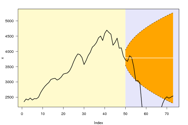
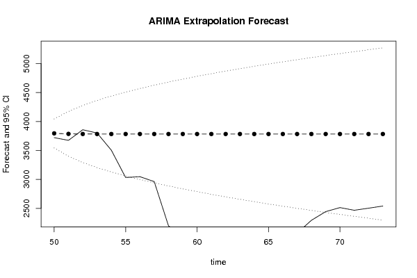
Title produced by software

ARIMA Forecasting

Date of computation

Tue, 21 Dec 2010 19:43:55 +0000

Cite this page as follows

Statistical Computations at FreeStatistics.org, Office for Research Development and Education, URL https://freestatistics.org/blog/index.php?v=date/2010/Dec/21/t1292960533ns8rzf1muxzrnap.htm/, Retrieved Thu, 16 May 2024 10:30:52 +0000

Statistical Computations at FreeStatistics.org, Office for Research Development and Education, URL https://freestatistics.org/blog/index.php?pk=113903, Retrieved Thu, 16 May 2024 10:30:52 +0000

QR Codes:

Paste this QR Code to cite your computation.

Original text written by user:

IsPrivate?

No (this computation is public)

User-defined keywords

Estimated Impact

112

Family? (F = Feedback message, R = changed R code, M = changed R Module, P = changed Parameters, D = changed Data)

-       [ARIMA Forecasting] [arima forecast] [2010-12-21 19:43:55] [06510e00f8d0c95cc2ff019b83c7c2eb] [Current]
- RMP     [Univariate Data Series] [] [2010-12-22 10:53:04] [ac04aa21811479ebaa189c580d7b203f] 
-    D      [Univariate Data Series] [ruwe data goudkoers] [2010-12-29 15:16:05] [ca50229b6b451ac8f5a30a9e3154d674] 
- RMPD      [Univariate Explorative Data Analysis] [Tutorial 2 Un EDA] [2011-12-23 19:36:45] [7d6928c5d92ed6ea67ea25577f8d26ae] 
- RMPD      [Variance Reduction Matrix] [] [2011-12-23 20:08:10] [7d6928c5d92ed6ea67ea25577f8d26ae] 
- RMPD      [(Partial) Autocorrelation Function] [] [2011-12-23 20:17:37] [7d6928c5d92ed6ea67ea25577f8d26ae] 
- RMPD      [(Partial) Autocorrelation Function] [] [2011-12-23 20:25:00] [7d6928c5d92ed6ea67ea25577f8d26ae] 
- RMPD      [(Partial) Autocorrelation Function] [] [2011-12-23 20:25:00] [7d6928c5d92ed6ea67ea25577f8d26ae] 
- RMPD      [(Partial) Autocorrelation Function] [] [2011-12-23 20:30:36] [7d6928c5d92ed6ea67ea25577f8d26ae] 
- RMPD      [Spectral Analysis] [] [2011-12-23 20:33:42] [7d6928c5d92ed6ea67ea25577f8d26ae] 
- RMPD      [Spectral Analysis] [] [2011-12-23 20:33:42] [7d6928c5d92ed6ea67ea25577f8d26ae] 

Feedback Forum

Post a new message

Dataseries X:

Download CSV

Histogram

Boxplots

Summary of computational transaction
Raw Input	view raw input (R code)
Raw Output	view raw output of R engine
Computing time	1 seconds
R Server	'Sir Ronald Aylmer Fisher' @ 193.190.124.24

\begin{tabular}{lllllllll}
\hline
Summary of computational transaction \tabularnewline
Raw Input & view raw input (R code)  \tabularnewline
Raw Output & view raw output of R engine  \tabularnewline
Computing time & 1 seconds \tabularnewline
R Server & 'Sir Ronald Aylmer Fisher' @ 193.190.124.24 \tabularnewline
\hline
\end{tabular}
%Source: https://freestatistics.org/blog/index.php?pk=113903&T=0

[TABLE]
[ROW][C]Summary of computational transaction[/C][/ROW]
[ROW][C]Raw Input[/C][C]view raw input (R code) [/C][/ROW]
[ROW][C]Raw Output[/C][C]view raw output of R engine [/C][/ROW]
[ROW][C]Computing time[/C][C]1 seconds[/C][/ROW]
[ROW][C]R Server[/C][C]'Sir Ronald Aylmer Fisher' @ 193.190.124.24[/C][/ROW]
[/TABLE]
Source: https://freestatistics.org/blog/index.php?pk=113903&T=0

Globally Unique Identifier (entire table): ba.freestatistics.org/blog/index.php?pk=113903&T=0

As an alternative you can also use a QR Code:

The GUIDs for individual cells are displayed in the table below:

Summary of computational transaction
Raw Input	view raw input (R code)
Raw Output	view raw output of R engine
Computing time	1 seconds
R Server	'Sir Ronald Aylmer Fisher' @ 193.190.124.24

Univariate ARIMA Extrapolation Forecast
time	Y[t]	F[t]	95% LB	95% UB	p-value(H0: Y[t] = F[t])	P(F[t]>Y[t-1])	P(F[t]>Y[t-s])	P(F[t]>Y[49])
37	4443.91	-	-	-	-	-	-	-
38	4502.64	-	-	-	-	-	-	-
39	4356.98	-	-	-	-	-	-	-
40	4591.27	-	-	-	-	-	-	-
41	4696.96	-	-	-	-	-	-	-
42	4621.4	-	-	-	-	-	-	-
43	4562.84	-	-	-	-	-	-	-
44	4202.52	-	-	-	-	-	-	-
45	4296.49	-	-	-	-	-	-	-
46	4435.23	-	-	-	-	-	-	-
47	4105.18	-	-	-	-	-	-	-
48	4116.68	-	-	-	-	-	-	-
49	3844.49	-	-	-	-	-	-	-
50	3720.98	3795.0781	3544.5761	4045.5801	0.281	0.3495	0	0.3495
51	3674.4	3786.1081	3398.3538	4173.8625	0.2862	0.629	0.002	0.384
52	3857.62	3784.4798	3291.6202	4277.3394	0.3856	0.6692	7e-04	0.4057
53	3801.06	3784.1842	3204.1999	4364.1685	0.4773	0.402	0.001	0.4193
54	3504.37	3784.1305	3128.3719	4439.8891	0.2015	0.4798	0.0062	0.4284
55	3032.6	3784.1208	3060.4584	4507.7831	0.0209	0.7757	0.0175	0.4351
56	3047.03	3784.119	2998.3961	4569.842	0.033	0.9696	0.1483	0.4401
57	2962.34	3784.1187	2940.8899	4627.3475	0.0281	0.9567	0.1168	0.4442
58	2197.82	3784.1186	2887.0627	4681.1746	3e-04	0.9637	0.0774	0.4475
59	2014.45	3784.1186	2836.2875	4731.9498	1e-04	0.9995	0.2534	0.4503
60	1862.83	3784.1186	2788.0973	4780.1399	1e-04	0.9998	0.2564	0.4527
61	1905.41	3784.1186	2742.1335	4826.1037	2e-04	0.9998	0.4548	0.4548
62	1810.99	3784.1186	2698.1133	4870.1239	2e-04	0.9997	0.5454	0.4566
63	1670.07	3784.1186	2655.8092	4912.428	1e-04	0.9997	0.5756	0.4582
64	1864.44	3784.1186	2615.0349	4953.2023	6e-04	0.9998	0.451	0.4597
65	2052.02	3784.1186	2575.6356	4992.6016	0.0025	0.9991	0.489	0.461
66	2029.6	3784.1186	2537.4809	5030.7564	0.0029	0.9968	0.67	0.4622
67	2070.83	3784.1186	2500.4597	5067.7776	0.0044	0.9963	0.8744	0.4633
68	2293.41	3784.1186	2464.4767	5103.7605	0.0134	0.9945	0.8632	0.4643
69	2443.27	3784.1186	2429.4492	5138.7881	0.0262	0.9845	0.8828	0.4652
70	2513.17	3784.1186	2395.3048	5172.9325	0.0364	0.9708	0.9874	0.4661
71	2466.92	3784.1186	2361.9799	5206.2573	0.0347	0.9601	0.9926	0.4668
72	2502.66	3784.1186	2329.4183	5238.8189	0.0421	0.962	0.9952	0.4676
73	2539.91	3784.1186	2297.5697	5270.6675	0.0505	0.9544	0.9934	0.4683

\begin{tabular}{lllllllll}
\hline
Univariate ARIMA Extrapolation Forecast \tabularnewline
time & Y[t] & F[t] & 95% LB & 95% UB & p-value(H0: Y[t] = F[t]) & P(F[t]>Y[t-1]) & P(F[t]>Y[t-s]) & P(F[t]>Y[49]) \tabularnewline
37 & 4443.91 & - & - & - & - & - & - & - \tabularnewline
38 & 4502.64 & - & - & - & - & - & - & - \tabularnewline
39 & 4356.98 & - & - & - & - & - & - & - \tabularnewline
40 & 4591.27 & - & - & - & - & - & - & - \tabularnewline
41 & 4696.96 & - & - & - & - & - & - & - \tabularnewline
42 & 4621.4 & - & - & - & - & - & - & - \tabularnewline
43 & 4562.84 & - & - & - & - & - & - & - \tabularnewline
44 & 4202.52 & - & - & - & - & - & - & - \tabularnewline
45 & 4296.49 & - & - & - & - & - & - & - \tabularnewline
46 & 4435.23 & - & - & - & - & - & - & - \tabularnewline
47 & 4105.18 & - & - & - & - & - & - & - \tabularnewline
48 & 4116.68 & - & - & - & - & - & - & - \tabularnewline
49 & 3844.49 & - & - & - & - & - & - & - \tabularnewline
50 & 3720.98 & 3795.0781 & 3544.5761 & 4045.5801 & 0.281 & 0.3495 & 0 & 0.3495 \tabularnewline
51 & 3674.4 & 3786.1081 & 3398.3538 & 4173.8625 & 0.2862 & 0.629 & 0.002 & 0.384 \tabularnewline
52 & 3857.62 & 3784.4798 & 3291.6202 & 4277.3394 & 0.3856 & 0.6692 & 7e-04 & 0.4057 \tabularnewline
53 & 3801.06 & 3784.1842 & 3204.1999 & 4364.1685 & 0.4773 & 0.402 & 0.001 & 0.4193 \tabularnewline
54 & 3504.37 & 3784.1305 & 3128.3719 & 4439.8891 & 0.2015 & 0.4798 & 0.0062 & 0.4284 \tabularnewline
55 & 3032.6 & 3784.1208 & 3060.4584 & 4507.7831 & 0.0209 & 0.7757 & 0.0175 & 0.4351 \tabularnewline
56 & 3047.03 & 3784.119 & 2998.3961 & 4569.842 & 0.033 & 0.9696 & 0.1483 & 0.4401 \tabularnewline
57 & 2962.34 & 3784.1187 & 2940.8899 & 4627.3475 & 0.0281 & 0.9567 & 0.1168 & 0.4442 \tabularnewline
58 & 2197.82 & 3784.1186 & 2887.0627 & 4681.1746 & 3e-04 & 0.9637 & 0.0774 & 0.4475 \tabularnewline
59 & 2014.45 & 3784.1186 & 2836.2875 & 4731.9498 & 1e-04 & 0.9995 & 0.2534 & 0.4503 \tabularnewline
60 & 1862.83 & 3784.1186 & 2788.0973 & 4780.1399 & 1e-04 & 0.9998 & 0.2564 & 0.4527 \tabularnewline
61 & 1905.41 & 3784.1186 & 2742.1335 & 4826.1037 & 2e-04 & 0.9998 & 0.4548 & 0.4548 \tabularnewline
62 & 1810.99 & 3784.1186 & 2698.1133 & 4870.1239 & 2e-04 & 0.9997 & 0.5454 & 0.4566 \tabularnewline
63 & 1670.07 & 3784.1186 & 2655.8092 & 4912.428 & 1e-04 & 0.9997 & 0.5756 & 0.4582 \tabularnewline
64 & 1864.44 & 3784.1186 & 2615.0349 & 4953.2023 & 6e-04 & 0.9998 & 0.451 & 0.4597 \tabularnewline
65 & 2052.02 & 3784.1186 & 2575.6356 & 4992.6016 & 0.0025 & 0.9991 & 0.489 & 0.461 \tabularnewline
66 & 2029.6 & 3784.1186 & 2537.4809 & 5030.7564 & 0.0029 & 0.9968 & 0.67 & 0.4622 \tabularnewline
67 & 2070.83 & 3784.1186 & 2500.4597 & 5067.7776 & 0.0044 & 0.9963 & 0.8744 & 0.4633 \tabularnewline
68 & 2293.41 & 3784.1186 & 2464.4767 & 5103.7605 & 0.0134 & 0.9945 & 0.8632 & 0.4643 \tabularnewline
69 & 2443.27 & 3784.1186 & 2429.4492 & 5138.7881 & 0.0262 & 0.9845 & 0.8828 & 0.4652 \tabularnewline
70 & 2513.17 & 3784.1186 & 2395.3048 & 5172.9325 & 0.0364 & 0.9708 & 0.9874 & 0.4661 \tabularnewline
71 & 2466.92 & 3784.1186 & 2361.9799 & 5206.2573 & 0.0347 & 0.9601 & 0.9926 & 0.4668 \tabularnewline
72 & 2502.66 & 3784.1186 & 2329.4183 & 5238.8189 & 0.0421 & 0.962 & 0.9952 & 0.4676 \tabularnewline
73 & 2539.91 & 3784.1186 & 2297.5697 & 5270.6675 & 0.0505 & 0.9544 & 0.9934 & 0.4683 \tabularnewline
\hline
\end{tabular}
%Source: https://freestatistics.org/blog/index.php?pk=113903&T=1

[TABLE]
[ROW][C]Univariate ARIMA Extrapolation Forecast[/C][/ROW]
[ROW][C]time[/C][C]Y[t][/C][C]F[t][/C][C]95% LB[/C][C]95% UB[/C][C]p-value(H0: Y[t] = F[t])[/C][C]P(F[t]>Y[t-1])[/C][C]P(F[t]>Y[t-s])[/C][C]P(F[t]>Y[49])[/C][/ROW]
[ROW][C]37[/C][C]4443.91[/C][C]-[/C][C]-[/C][C]-[/C][C]-[/C][C]-[/C][C]-[/C][C]-[/C][/ROW]
[ROW][C]38[/C][C]4502.64[/C][C]-[/C][C]-[/C][C]-[/C][C]-[/C][C]-[/C][C]-[/C][C]-[/C][/ROW]
[ROW][C]39[/C][C]4356.98[/C][C]-[/C][C]-[/C][C]-[/C][C]-[/C][C]-[/C][C]-[/C][C]-[/C][/ROW]
[ROW][C]40[/C][C]4591.27[/C][C]-[/C][C]-[/C][C]-[/C][C]-[/C][C]-[/C][C]-[/C][C]-[/C][/ROW]
[ROW][C]41[/C][C]4696.96[/C][C]-[/C][C]-[/C][C]-[/C][C]-[/C][C]-[/C][C]-[/C][C]-[/C][/ROW]
[ROW][C]42[/C][C]4621.4[/C][C]-[/C][C]-[/C][C]-[/C][C]-[/C][C]-[/C][C]-[/C][C]-[/C][/ROW]
[ROW][C]43[/C][C]4562.84[/C][C]-[/C][C]-[/C][C]-[/C][C]-[/C][C]-[/C][C]-[/C][C]-[/C][/ROW]
[ROW][C]44[/C][C]4202.52[/C][C]-[/C][C]-[/C][C]-[/C][C]-[/C][C]-[/C][C]-[/C][C]-[/C][/ROW]
[ROW][C]45[/C][C]4296.49[/C][C]-[/C][C]-[/C][C]-[/C][C]-[/C][C]-[/C][C]-[/C][C]-[/C][/ROW]
[ROW][C]46[/C][C]4435.23[/C][C]-[/C][C]-[/C][C]-[/C][C]-[/C][C]-[/C][C]-[/C][C]-[/C][/ROW]
[ROW][C]47[/C][C]4105.18[/C][C]-[/C][C]-[/C][C]-[/C][C]-[/C][C]-[/C][C]-[/C][C]-[/C][/ROW]
[ROW][C]48[/C][C]4116.68[/C][C]-[/C][C]-[/C][C]-[/C][C]-[/C][C]-[/C][C]-[/C][C]-[/C][/ROW]
[ROW][C]49[/C][C]3844.49[/C][C]-[/C][C]-[/C][C]-[/C][C]-[/C][C]-[/C][C]-[/C][C]-[/C][/ROW]
[ROW][C]50[/C][C]3720.98[/C][C]3795.0781[/C][C]3544.5761[/C][C]4045.5801[/C][C]0.281[/C][C]0.3495[/C][C]0[/C][C]0.3495[/C][/ROW]
[ROW][C]51[/C][C]3674.4[/C][C]3786.1081[/C][C]3398.3538[/C][C]4173.8625[/C][C]0.2862[/C][C]0.629[/C][C]0.002[/C][C]0.384[/C][/ROW]
[ROW][C]52[/C][C]3857.62[/C][C]3784.4798[/C][C]3291.6202[/C][C]4277.3394[/C][C]0.3856[/C][C]0.6692[/C][C]7e-04[/C][C]0.4057[/C][/ROW]
[ROW][C]53[/C][C]3801.06[/C][C]3784.1842[/C][C]3204.1999[/C][C]4364.1685[/C][C]0.4773[/C][C]0.402[/C][C]0.001[/C][C]0.4193[/C][/ROW]
[ROW][C]54[/C][C]3504.37[/C][C]3784.1305[/C][C]3128.3719[/C][C]4439.8891[/C][C]0.2015[/C][C]0.4798[/C][C]0.0062[/C][C]0.4284[/C][/ROW]
[ROW][C]55[/C][C]3032.6[/C][C]3784.1208[/C][C]3060.4584[/C][C]4507.7831[/C][C]0.0209[/C][C]0.7757[/C][C]0.0175[/C][C]0.4351[/C][/ROW]
[ROW][C]56[/C][C]3047.03[/C][C]3784.119[/C][C]2998.3961[/C][C]4569.842[/C][C]0.033[/C][C]0.9696[/C][C]0.1483[/C][C]0.4401[/C][/ROW]
[ROW][C]57[/C][C]2962.34[/C][C]3784.1187[/C][C]2940.8899[/C][C]4627.3475[/C][C]0.0281[/C][C]0.9567[/C][C]0.1168[/C][C]0.4442[/C][/ROW]
[ROW][C]58[/C][C]2197.82[/C][C]3784.1186[/C][C]2887.0627[/C][C]4681.1746[/C][C]3e-04[/C][C]0.9637[/C][C]0.0774[/C][C]0.4475[/C][/ROW]
[ROW][C]59[/C][C]2014.45[/C][C]3784.1186[/C][C]2836.2875[/C][C]4731.9498[/C][C]1e-04[/C][C]0.9995[/C][C]0.2534[/C][C]0.4503[/C][/ROW]
[ROW][C]60[/C][C]1862.83[/C][C]3784.1186[/C][C]2788.0973[/C][C]4780.1399[/C][C]1e-04[/C][C]0.9998[/C][C]0.2564[/C][C]0.4527[/C][/ROW]
[ROW][C]61[/C][C]1905.41[/C][C]3784.1186[/C][C]2742.1335[/C][C]4826.1037[/C][C]2e-04[/C][C]0.9998[/C][C]0.4548[/C][C]0.4548[/C][/ROW]
[ROW][C]62[/C][C]1810.99[/C][C]3784.1186[/C][C]2698.1133[/C][C]4870.1239[/C][C]2e-04[/C][C]0.9997[/C][C]0.5454[/C][C]0.4566[/C][/ROW]
[ROW][C]63[/C][C]1670.07[/C][C]3784.1186[/C][C]2655.8092[/C][C]4912.428[/C][C]1e-04[/C][C]0.9997[/C][C]0.5756[/C][C]0.4582[/C][/ROW]
[ROW][C]64[/C][C]1864.44[/C][C]3784.1186[/C][C]2615.0349[/C][C]4953.2023[/C][C]6e-04[/C][C]0.9998[/C][C]0.451[/C][C]0.4597[/C][/ROW]
[ROW][C]65[/C][C]2052.02[/C][C]3784.1186[/C][C]2575.6356[/C][C]4992.6016[/C][C]0.0025[/C][C]0.9991[/C][C]0.489[/C][C]0.461[/C][/ROW]
[ROW][C]66[/C][C]2029.6[/C][C]3784.1186[/C][C]2537.4809[/C][C]5030.7564[/C][C]0.0029[/C][C]0.9968[/C][C]0.67[/C][C]0.4622[/C][/ROW]
[ROW][C]67[/C][C]2070.83[/C][C]3784.1186[/C][C]2500.4597[/C][C]5067.7776[/C][C]0.0044[/C][C]0.9963[/C][C]0.8744[/C][C]0.4633[/C][/ROW]
[ROW][C]68[/C][C]2293.41[/C][C]3784.1186[/C][C]2464.4767[/C][C]5103.7605[/C][C]0.0134[/C][C]0.9945[/C][C]0.8632[/C][C]0.4643[/C][/ROW]
[ROW][C]69[/C][C]2443.27[/C][C]3784.1186[/C][C]2429.4492[/C][C]5138.7881[/C][C]0.0262[/C][C]0.9845[/C][C]0.8828[/C][C]0.4652[/C][/ROW]
[ROW][C]70[/C][C]2513.17[/C][C]3784.1186[/C][C]2395.3048[/C][C]5172.9325[/C][C]0.0364[/C][C]0.9708[/C][C]0.9874[/C][C]0.4661[/C][/ROW]
[ROW][C]71[/C][C]2466.92[/C][C]3784.1186[/C][C]2361.9799[/C][C]5206.2573[/C][C]0.0347[/C][C]0.9601[/C][C]0.9926[/C][C]0.4668[/C][/ROW]
[ROW][C]72[/C][C]2502.66[/C][C]3784.1186[/C][C]2329.4183[/C][C]5238.8189[/C][C]0.0421[/C][C]0.962[/C][C]0.9952[/C][C]0.4676[/C][/ROW]
[ROW][C]73[/C][C]2539.91[/C][C]3784.1186[/C][C]2297.5697[/C][C]5270.6675[/C][C]0.0505[/C][C]0.9544[/C][C]0.9934[/C][C]0.4683[/C][/ROW]
[/TABLE]
Source: https://freestatistics.org/blog/index.php?pk=113903&T=1

Globally Unique Identifier (entire table): ba.freestatistics.org/blog/index.php?pk=113903&T=1

As an alternative you can also use a QR Code:

The GUIDs for individual cells are displayed in the table below:

Univariate ARIMA Extrapolation Forecast
time	Y[t]	F[t]	95% LB	95% UB	p-value(H0: Y[t] = F[t])	P(F[t]>Y[t-1])	P(F[t]>Y[t-s])	P(F[t]>Y[49])
37	4443.91	-	-	-	-	-	-	-
38	4502.64	-	-	-	-	-	-	-
39	4356.98	-	-	-	-	-	-	-
40	4591.27	-	-	-	-	-	-	-
41	4696.96	-	-	-	-	-	-	-
42	4621.4	-	-	-	-	-	-	-
43	4562.84	-	-	-	-	-	-	-
44	4202.52	-	-	-	-	-	-	-
45	4296.49	-	-	-	-	-	-	-
46	4435.23	-	-	-	-	-	-	-
47	4105.18	-	-	-	-	-	-	-
48	4116.68	-	-	-	-	-	-	-
49	3844.49	-	-	-	-	-	-	-
50	3720.98	3795.0781	3544.5761	4045.5801	0.281	0.3495	0	0.3495
51	3674.4	3786.1081	3398.3538	4173.8625	0.2862	0.629	0.002	0.384
52	3857.62	3784.4798	3291.6202	4277.3394	0.3856	0.6692	7e-04	0.4057
53	3801.06	3784.1842	3204.1999	4364.1685	0.4773	0.402	0.001	0.4193
54	3504.37	3784.1305	3128.3719	4439.8891	0.2015	0.4798	0.0062	0.4284
55	3032.6	3784.1208	3060.4584	4507.7831	0.0209	0.7757	0.0175	0.4351
56	3047.03	3784.119	2998.3961	4569.842	0.033	0.9696	0.1483	0.4401
57	2962.34	3784.1187	2940.8899	4627.3475	0.0281	0.9567	0.1168	0.4442
58	2197.82	3784.1186	2887.0627	4681.1746	3e-04	0.9637	0.0774	0.4475
59	2014.45	3784.1186	2836.2875	4731.9498	1e-04	0.9995	0.2534	0.4503
60	1862.83	3784.1186	2788.0973	4780.1399	1e-04	0.9998	0.2564	0.4527
61	1905.41	3784.1186	2742.1335	4826.1037	2e-04	0.9998	0.4548	0.4548
62	1810.99	3784.1186	2698.1133	4870.1239	2e-04	0.9997	0.5454	0.4566
63	1670.07	3784.1186	2655.8092	4912.428	1e-04	0.9997	0.5756	0.4582
64	1864.44	3784.1186	2615.0349	4953.2023	6e-04	0.9998	0.451	0.4597
65	2052.02	3784.1186	2575.6356	4992.6016	0.0025	0.9991	0.489	0.461
66	2029.6	3784.1186	2537.4809	5030.7564	0.0029	0.9968	0.67	0.4622
67	2070.83	3784.1186	2500.4597	5067.7776	0.0044	0.9963	0.8744	0.4633
68	2293.41	3784.1186	2464.4767	5103.7605	0.0134	0.9945	0.8632	0.4643
69	2443.27	3784.1186	2429.4492	5138.7881	0.0262	0.9845	0.8828	0.4652
70	2513.17	3784.1186	2395.3048	5172.9325	0.0364	0.9708	0.9874	0.4661
71	2466.92	3784.1186	2361.9799	5206.2573	0.0347	0.9601	0.9926	0.4668
72	2502.66	3784.1186	2329.4183	5238.8189	0.0421	0.962	0.9952	0.4676
73	2539.91	3784.1186	2297.5697	5270.6675	0.0505	0.9544	0.9934	0.4683

Univariate ARIMA Extrapolation Forecast Performance
time	% S.E.	PE	MAPE	Sq.E	MSE	RMSE
50	0.0337	-0.0195	0	5490.5302	0	0
51	0.0523	-0.0295	0.0245	12478.7102	8984.6202	94.7872
52	0.0664	0.0193	0.0228	5349.4905	7772.9103	88.1641
53	0.0782	0.0045	0.0182	284.7931	5900.881	76.8172
54	0.0884	-0.0739	0.0293	78265.9504	20373.8949	142.7372
55	0.0976	-0.1986	0.0576	564783.4855	111108.8267	333.3299
56	0.1059	-0.1948	0.0772	543300.2137	172850.4534	415.7529
57	0.1137	-0.2172	0.0947	675320.2192	235659.1741	485.4474
58	0.1209	-0.4192	0.1307	2516343.3565	489068.5277	699.3343
59	0.1278	-0.4677	0.1644	3131727.037	753334.3786	867.9484
60	0.1343	-0.5077	0.1956	3691349.9674	1020426.7049	1010.1617
61	0.1405	-0.4965	0.2207	3529546.0835	1229519.9864	1108.8372
62	0.1464	-0.5214	0.2438	3893236.5557	1434421.261	1197.6733
63	0.1521	-0.5587	0.2663	4469201.5726	1651191.2833	1284.9869
64	0.1576	-0.5073	0.2824	3685166.0085	1786789.5983	1336.7085
65	0.1629	-0.4577	0.2933	3000165.6334	1862625.6005	1364.7804
66	0.1681	-0.4637	0.3034	3078335.592	1934137.9529	1390.7329
67	0.1731	-0.4528	0.3117	2935357.8994	1989761.2833	1410.589
68	0.1779	-0.3939	0.316	2222212.1932	2001995.5417	1414.9189
69	0.1826	-0.3543	0.3179	1797875.0249	1991789.5159	1411.3077
70	0.1873	-0.3359	0.3188	1615310.3976	1973861.9388	1404.942
71	0.1917	-0.3481	0.3201	1735012.2076	1963005.1328	1401.0729
72	0.1961	-0.3386	0.3209	1642136.1977	1949054.3096	1396.0854
73	0.2004	-0.3288	0.3212	1548055.093	1932346.0089	1390.0885

\begin{tabular}{lllllllll}
\hline
Univariate ARIMA Extrapolation Forecast Performance \tabularnewline
time & % S.E. & PE & MAPE & Sq.E & MSE & RMSE \tabularnewline
50 & 0.0337 & -0.0195 & 0 & 5490.5302 & 0 & 0 \tabularnewline
51 & 0.0523 & -0.0295 & 0.0245 & 12478.7102 & 8984.6202 & 94.7872 \tabularnewline
52 & 0.0664 & 0.0193 & 0.0228 & 5349.4905 & 7772.9103 & 88.1641 \tabularnewline
53 & 0.0782 & 0.0045 & 0.0182 & 284.7931 & 5900.881 & 76.8172 \tabularnewline
54 & 0.0884 & -0.0739 & 0.0293 & 78265.9504 & 20373.8949 & 142.7372 \tabularnewline
55 & 0.0976 & -0.1986 & 0.0576 & 564783.4855 & 111108.8267 & 333.3299 \tabularnewline
56 & 0.1059 & -0.1948 & 0.0772 & 543300.2137 & 172850.4534 & 415.7529 \tabularnewline
57 & 0.1137 & -0.2172 & 0.0947 & 675320.2192 & 235659.1741 & 485.4474 \tabularnewline
58 & 0.1209 & -0.4192 & 0.1307 & 2516343.3565 & 489068.5277 & 699.3343 \tabularnewline
59 & 0.1278 & -0.4677 & 0.1644 & 3131727.037 & 753334.3786 & 867.9484 \tabularnewline
60 & 0.1343 & -0.5077 & 0.1956 & 3691349.9674 & 1020426.7049 & 1010.1617 \tabularnewline
61 & 0.1405 & -0.4965 & 0.2207 & 3529546.0835 & 1229519.9864 & 1108.8372 \tabularnewline
62 & 0.1464 & -0.5214 & 0.2438 & 3893236.5557 & 1434421.261 & 1197.6733 \tabularnewline
63 & 0.1521 & -0.5587 & 0.2663 & 4469201.5726 & 1651191.2833 & 1284.9869 \tabularnewline
64 & 0.1576 & -0.5073 & 0.2824 & 3685166.0085 & 1786789.5983 & 1336.7085 \tabularnewline
65 & 0.1629 & -0.4577 & 0.2933 & 3000165.6334 & 1862625.6005 & 1364.7804 \tabularnewline
66 & 0.1681 & -0.4637 & 0.3034 & 3078335.592 & 1934137.9529 & 1390.7329 \tabularnewline
67 & 0.1731 & -0.4528 & 0.3117 & 2935357.8994 & 1989761.2833 & 1410.589 \tabularnewline
68 & 0.1779 & -0.3939 & 0.316 & 2222212.1932 & 2001995.5417 & 1414.9189 \tabularnewline
69 & 0.1826 & -0.3543 & 0.3179 & 1797875.0249 & 1991789.5159 & 1411.3077 \tabularnewline
70 & 0.1873 & -0.3359 & 0.3188 & 1615310.3976 & 1973861.9388 & 1404.942 \tabularnewline
71 & 0.1917 & -0.3481 & 0.3201 & 1735012.2076 & 1963005.1328 & 1401.0729 \tabularnewline
72 & 0.1961 & -0.3386 & 0.3209 & 1642136.1977 & 1949054.3096 & 1396.0854 \tabularnewline
73 & 0.2004 & -0.3288 & 0.3212 & 1548055.093 & 1932346.0089 & 1390.0885 \tabularnewline
\hline
\end{tabular}
%Source: https://freestatistics.org/blog/index.php?pk=113903&T=2

[TABLE]
[ROW][C]Univariate ARIMA Extrapolation Forecast Performance[/C][/ROW]
[ROW][C]time[/C][C]% S.E.[/C][C]PE[/C][C]MAPE[/C][C]Sq.E[/C][C]MSE[/C][C]RMSE[/C][/ROW]
[ROW][C]50[/C][C]0.0337[/C][C]-0.0195[/C][C]0[/C][C]5490.5302[/C][C]0[/C][C]0[/C][/ROW]
[ROW][C]51[/C][C]0.0523[/C][C]-0.0295[/C][C]0.0245[/C][C]12478.7102[/C][C]8984.6202[/C][C]94.7872[/C][/ROW]
[ROW][C]52[/C][C]0.0664[/C][C]0.0193[/C][C]0.0228[/C][C]5349.4905[/C][C]7772.9103[/C][C]88.1641[/C][/ROW]
[ROW][C]53[/C][C]0.0782[/C][C]0.0045[/C][C]0.0182[/C][C]284.7931[/C][C]5900.881[/C][C]76.8172[/C][/ROW]
[ROW][C]54[/C][C]0.0884[/C][C]-0.0739[/C][C]0.0293[/C][C]78265.9504[/C][C]20373.8949[/C][C]142.7372[/C][/ROW]
[ROW][C]55[/C][C]0.0976[/C][C]-0.1986[/C][C]0.0576[/C][C]564783.4855[/C][C]111108.8267[/C][C]333.3299[/C][/ROW]
[ROW][C]56[/C][C]0.1059[/C][C]-0.1948[/C][C]0.0772[/C][C]543300.2137[/C][C]172850.4534[/C][C]415.7529[/C][/ROW]
[ROW][C]57[/C][C]0.1137[/C][C]-0.2172[/C][C]0.0947[/C][C]675320.2192[/C][C]235659.1741[/C][C]485.4474[/C][/ROW]
[ROW][C]58[/C][C]0.1209[/C][C]-0.4192[/C][C]0.1307[/C][C]2516343.3565[/C][C]489068.5277[/C][C]699.3343[/C][/ROW]
[ROW][C]59[/C][C]0.1278[/C][C]-0.4677[/C][C]0.1644[/C][C]3131727.037[/C][C]753334.3786[/C][C]867.9484[/C][/ROW]
[ROW][C]60[/C][C]0.1343[/C][C]-0.5077[/C][C]0.1956[/C][C]3691349.9674[/C][C]1020426.7049[/C][C]1010.1617[/C][/ROW]
[ROW][C]61[/C][C]0.1405[/C][C]-0.4965[/C][C]0.2207[/C][C]3529546.0835[/C][C]1229519.9864[/C][C]1108.8372[/C][/ROW]
[ROW][C]62[/C][C]0.1464[/C][C]-0.5214[/C][C]0.2438[/C][C]3893236.5557[/C][C]1434421.261[/C][C]1197.6733[/C][/ROW]
[ROW][C]63[/C][C]0.1521[/C][C]-0.5587[/C][C]0.2663[/C][C]4469201.5726[/C][C]1651191.2833[/C][C]1284.9869[/C][/ROW]
[ROW][C]64[/C][C]0.1576[/C][C]-0.5073[/C][C]0.2824[/C][C]3685166.0085[/C][C]1786789.5983[/C][C]1336.7085[/C][/ROW]
[ROW][C]65[/C][C]0.1629[/C][C]-0.4577[/C][C]0.2933[/C][C]3000165.6334[/C][C]1862625.6005[/C][C]1364.7804[/C][/ROW]
[ROW][C]66[/C][C]0.1681[/C][C]-0.4637[/C][C]0.3034[/C][C]3078335.592[/C][C]1934137.9529[/C][C]1390.7329[/C][/ROW]
[ROW][C]67[/C][C]0.1731[/C][C]-0.4528[/C][C]0.3117[/C][C]2935357.8994[/C][C]1989761.2833[/C][C]1410.589[/C][/ROW]
[ROW][C]68[/C][C]0.1779[/C][C]-0.3939[/C][C]0.316[/C][C]2222212.1932[/C][C]2001995.5417[/C][C]1414.9189[/C][/ROW]
[ROW][C]69[/C][C]0.1826[/C][C]-0.3543[/C][C]0.3179[/C][C]1797875.0249[/C][C]1991789.5159[/C][C]1411.3077[/C][/ROW]
[ROW][C]70[/C][C]0.1873[/C][C]-0.3359[/C][C]0.3188[/C][C]1615310.3976[/C][C]1973861.9388[/C][C]1404.942[/C][/ROW]
[ROW][C]71[/C][C]0.1917[/C][C]-0.3481[/C][C]0.3201[/C][C]1735012.2076[/C][C]1963005.1328[/C][C]1401.0729[/C][/ROW]
[ROW][C]72[/C][C]0.1961[/C][C]-0.3386[/C][C]0.3209[/C][C]1642136.1977[/C][C]1949054.3096[/C][C]1396.0854[/C][/ROW]
[ROW][C]73[/C][C]0.2004[/C][C]-0.3288[/C][C]0.3212[/C][C]1548055.093[/C][C]1932346.0089[/C][C]1390.0885[/C][/ROW]
[/TABLE]
Source: https://freestatistics.org/blog/index.php?pk=113903&T=2

Globally Unique Identifier (entire table): ba.freestatistics.org/blog/index.php?pk=113903&T=2

As an alternative you can also use a QR Code:

The GUIDs for individual cells are displayed in the table below:

Univariate ARIMA Extrapolation Forecast Performance
time	% S.E.	PE	MAPE	Sq.E	MSE	RMSE
50	0.0337	-0.0195	0	5490.5302	0	0
51	0.0523	-0.0295	0.0245	12478.7102	8984.6202	94.7872
52	0.0664	0.0193	0.0228	5349.4905	7772.9103	88.1641
53	0.0782	0.0045	0.0182	284.7931	5900.881	76.8172
54	0.0884	-0.0739	0.0293	78265.9504	20373.8949	142.7372
55	0.0976	-0.1986	0.0576	564783.4855	111108.8267	333.3299
56	0.1059	-0.1948	0.0772	543300.2137	172850.4534	415.7529
57	0.1137	-0.2172	0.0947	675320.2192	235659.1741	485.4474
58	0.1209	-0.4192	0.1307	2516343.3565	489068.5277	699.3343
59	0.1278	-0.4677	0.1644	3131727.037	753334.3786	867.9484
60	0.1343	-0.5077	0.1956	3691349.9674	1020426.7049	1010.1617
61	0.1405	-0.4965	0.2207	3529546.0835	1229519.9864	1108.8372
62	0.1464	-0.5214	0.2438	3893236.5557	1434421.261	1197.6733
63	0.1521	-0.5587	0.2663	4469201.5726	1651191.2833	1284.9869
64	0.1576	-0.5073	0.2824	3685166.0085	1786789.5983	1336.7085
65	0.1629	-0.4577	0.2933	3000165.6334	1862625.6005	1364.7804
66	0.1681	-0.4637	0.3034	3078335.592	1934137.9529	1390.7329
67	0.1731	-0.4528	0.3117	2935357.8994	1989761.2833	1410.589
68	0.1779	-0.3939	0.316	2222212.1932	2001995.5417	1414.9189
69	0.1826	-0.3543	0.3179	1797875.0249	1991789.5159	1411.3077
70	0.1873	-0.3359	0.3188	1615310.3976	1973861.9388	1404.942
71	0.1917	-0.3481	0.3201	1735012.2076	1963005.1328	1401.0729
72	0.1961	-0.3386	0.3209	1642136.1977	1949054.3096	1396.0854
73	0.2004	-0.3288	0.3212	1548055.093	1932346.0089	1390.0885

Figure 1

PNG link

Postscript link

PDF link

Figure 2

PNG link

Postscript link

PDF link

Parameters (Session):

par1 = 24 ; par2 = 1 ; par3 = 1 ; par4 = 0 ; par5 = 12 ; par6 = 1 ; par7 = 0 ; par8 = 0 ; par9 = 0 ; par10 = FALSE ;

Parameters (R input):

par1 = 24 ; par2 = 1 ; par3 = 1 ; par4 = 0 ; par5 = 12 ; par6 = 1 ; par7 = 0 ; par8 = 0 ; par9 = 0 ; par10 = FALSE ;

R code (references can be found in the software module):

par1 <- as.numeric(par1) #cut off periods
par2 <- as.numeric(par2) #lambda
par3 <- as.numeric(par3) #degree of non-seasonal differencing
par4 <- as.numeric(par4) #degree of seasonal differencing
par5 <- as.numeric(par5) #seasonal period
par6 <- as.numeric(par6) #p
par7 <- as.numeric(par7) #q
par8 <- as.numeric(par8) #P
par9 <- as.numeric(par9) #Q
if (par10 == 'TRUE') par10 <- TRUE
if (par10 == 'FALSE') par10 <- FALSE
if (par2 == 0) x <- log(x)
if (par2 != 0) x <- x^par2
lx <- length(x)
first <- lx - 2*par1
nx <- lx - par1
nx1 <- nx + 1
fx <- lx - nx
if (fx < 1) {
fx <- par5
nx1 <- lx + fx - 1
first <- lx - 2*fx
}
first <- 1
if (fx < 3) fx <- round(lx/10,0)
(arima.out <- arima(x[1:nx], order=c(par6,par3,par7), seasonal=list(order=c(par8,par4,par9), period=par5), include.mean=par10, method='ML'))
(forecast <- predict(arima.out,par1))
(lb <- forecast$pred - 1.96 * forecast$se)
(ub <- forecast$pred + 1.96 * forecast$se)
if (par2 == 0) {
x <- exp(x)
forecast$pred <- exp(forecast$pred)
lb <- exp(lb)
ub <- exp(ub)
}
if (par2 != 0) {
x <- x^(1/par2)
forecast$pred <- forecast$pred^(1/par2)
lb <- lb^(1/par2)
ub <- ub^(1/par2)
}
if (par2 < 0) {
olb <- lb
lb <- ub
ub <- olb
}
(actandfor <- c(x[1:nx], forecast$pred))
(perc.se <- (ub-forecast$pred)/1.96/forecast$pred)
bitmap(file='test1.png')
opar <- par(mar=c(4,4,2,2),las=1)
ylim <- c( min(x[first:nx],lb), max(x[first:nx],ub))
plot(x,ylim=ylim,type='n',xlim=c(first,lx))
usr <- par('usr')
rect(usr[1],usr[3],nx+1,usr[4],border=NA,col='lemonchiffon')
rect(nx1,usr[3],usr[2],usr[4],border=NA,col='lavender')
abline(h= (-3:3)*2 , col ='gray', lty =3)
polygon( c(nx1:lx,lx:nx1), c(lb,rev(ub)), col = 'orange', lty=2,border=NA)
lines(nx1:lx, lb , lty=2)
lines(nx1:lx, ub , lty=2)
lines(x, lwd=2)
lines(nx1:lx, forecast$pred , lwd=2 , col ='white')
box()
par(opar)
dev.off()
prob.dec <- array(NA, dim=fx)
prob.sdec <- array(NA, dim=fx)
prob.ldec <- array(NA, dim=fx)
prob.pval <- array(NA, dim=fx)
perf.pe <- array(0, dim=fx)
perf.mape <- array(0, dim=fx)
perf.mape1 <- array(0, dim=fx)
perf.se <- array(0, dim=fx)
perf.mse <- array(0, dim=fx)
perf.mse1 <- array(0, dim=fx)
perf.rmse <- array(0, dim=fx)
for (i in 1:fx) {
locSD <- (ub[i] - forecast$pred[i]) / 1.96
perf.pe[i] = (x[nx+i] - forecast$pred[i]) / forecast$pred[i]
perf.se[i] = (x[nx+i] - forecast$pred[i])^2
prob.dec[i] = pnorm((x[nx+i-1] - forecast$pred[i]) / locSD)
prob.sdec[i] = pnorm((x[nx+i-par5] - forecast$pred[i]) / locSD)
prob.ldec[i] = pnorm((x[nx] - forecast$pred[i]) / locSD)
prob.pval[i] = pnorm(abs(x[nx+i] - forecast$pred[i]) / locSD)
}
perf.mape[1] = abs(perf.pe[1])
perf.mse[1] = abs(perf.se[1])
for (i in 2:fx) {
perf.mape[i] = perf.mape[i-1] + abs(perf.pe[i])
perf.mape1[i] = perf.mape[i] / i
perf.mse[i] = perf.mse[i-1] + perf.se[i]
perf.mse1[i] = perf.mse[i] / i
}
perf.rmse = sqrt(perf.mse1)
bitmap(file='test2.png')
plot(forecast$pred, pch=19, type='b',main='ARIMA Extrapolation Forecast', ylab='Forecast and 95% CI', xlab='time',ylim=c(min(lb),max(ub)))
dum <- forecast$pred
dum[1:par1] <- x[(nx+1):lx]
lines(dum, lty=1)
lines(ub,lty=3)
lines(lb,lty=3)
dev.off()
load(file='createtable')
a<-table.start()
a<-table.row.start(a)
a<-table.element(a,'Univariate ARIMA Extrapolation Forecast',9,TRUE)
a<-table.row.end(a)
a<-table.row.start(a)
a<-table.element(a,'time',1,header=TRUE)
a<-table.element(a,'Y[t]',1,header=TRUE)
a<-table.element(a,'F[t]',1,header=TRUE)
a<-table.element(a,'95% LB',1,header=TRUE)
a<-table.element(a,'95% UB',1,header=TRUE)
a<-table.element(a,'p-value
(H0: Y[t] = F[t])',1,header=TRUE)
a<-table.element(a,'P(F[t]>Y[t-1])',1,header=TRUE)
a<-table.element(a,'P(F[t]>Y[t-s])',1,header=TRUE)
mylab <- paste('P(F[t]>Y[',nx,sep='')
mylab <- paste(mylab,'])',sep='')
a<-table.element(a,mylab,1,header=TRUE)
a<-table.row.end(a)
for (i in (nx-par5):nx) {
a<-table.row.start(a)
a<-table.element(a,i,header=TRUE)
a<-table.element(a,x[i])
a<-table.element(a,'-')
a<-table.element(a,'-')
a<-table.element(a,'-')
a<-table.element(a,'-')
a<-table.element(a,'-')
a<-table.element(a,'-')
a<-table.element(a,'-')
a<-table.row.end(a)
}
for (i in 1:fx) {
a<-table.row.start(a)
a<-table.element(a,nx+i,header=TRUE)
a<-table.element(a,round(x[nx+i],4))
a<-table.element(a,round(forecast$pred[i],4))
a<-table.element(a,round(lb[i],4))
a<-table.element(a,round(ub[i],4))
a<-table.element(a,round((1-prob.pval[i]),4))
a<-table.element(a,round((1-prob.dec[i]),4))
a<-table.element(a,round((1-prob.sdec[i]),4))
a<-table.element(a,round((1-prob.ldec[i]),4))
a<-table.row.end(a)
}
a<-table.end(a)
table.save(a,file='mytable.tab')
a<-table.start()
a<-table.row.start(a)
a<-table.element(a,'Univariate ARIMA Extrapolation Forecast Performance',7,TRUE)
a<-table.row.end(a)
a<-table.row.start(a)
a<-table.element(a,'time',1,header=TRUE)
a<-table.element(a,'% S.E.',1,header=TRUE)
a<-table.element(a,'PE',1,header=TRUE)
a<-table.element(a,'MAPE',1,header=TRUE)
a<-table.element(a,'Sq.E',1,header=TRUE)
a<-table.element(a,'MSE',1,header=TRUE)
a<-table.element(a,'RMSE',1,header=TRUE)
a<-table.row.end(a)
for (i in 1:fx) {
a<-table.row.start(a)
a<-table.element(a,nx+i,header=TRUE)
a<-table.element(a,round(perc.se[i],4))
a<-table.element(a,round(perf.pe[i],4))
a<-table.element(a,round(perf.mape1[i],4))
a<-table.element(a,round(perf.se[i],4))
a<-table.element(a,round(perf.mse1[i],4))
a<-table.element(a,round(perf.rmse[i],4))
a<-table.row.end(a)
}
a<-table.end(a)
table.save(a,file='mytable1.tab')

Free Statistics

Description of Statistical Computation

Tree of Dependent Computations

Dataset

Tables (Output of Computation)

Figures (Output of Computation)

Input Parameters & R Code