totaal verband huwelijken

*The author of this computation has been verified*

R Software Module: /rwasp_multipleregression.wasp (opens new window with default values)

Title produced by software: Multiple Regression

Date of computation: Tue, 21 Dec 2010 16:56:19 +0000

Cite this page as follows:

Statistical Computations at FreeStatistics.org, Office for Research Development and Education, URL http://www.freestatistics.org/blog/date/2010/Dec/21/t1292950510ohsghaiz6avqf9p.htm/, Retrieved Tue, 21 Dec 2010 17:55:13 +0100

BibTeX entries for LaTeX users:

@Manual{KEY, author = {{YOUR NAME}}, publisher = {Office for Research Development and Education}, title = {Statistical Computations at FreeStatistics.org, URL http://www.freestatistics.org/blog/date/2010/Dec/21/t1292950510ohsghaiz6avqf9p.htm/}, year = {2010}, } @Manual{R, title = {R: A Language and Environment for Statistical Computing}, author = {{R Development Core Team}}, organization = {R Foundation for Statistical Computing}, address = {Vienna, Austria}, year = {2010}, note = {{ISBN} 3-900051-07-0}, url = {http://www.R-project.org}, }

Original text written by user:

IsPrivate?

No (this computation is public)

User-defined keywords:

Dataseries X:

» Textbox « » Textfile « » CSV «

3111 5140 17153 2.5 766 332 2.4 3995 4749 15579 1.8 294 369 2.4 5245 3635 16755 7.3 235 384 2.4 5588 4305 16585 9.9 462 373 2.1 10681 5805 16572 13.2 919 378 2 10516 4260 16325 17.8 346 426 2 7496 3869 17913 18.8 298 423 2.1 9935 7325 17572 19.3 92 397 2.1 10249 9280 17338 13.9 516 422 2 6271 6222 17087 7.5 843 409 2 3616 3272 15864 8 395 430 2 3724 7598 15554 4 961 412 1.7 2886 1345 16229 3.6 1231 470 1.3 3318 1900 15180 4.8 794 491 1.2 4166 1480 16215 5.9 420 504 1.1 6401 1472 15801 10.4 331 484 1.4 9209 3823 15751 12.3 312 474 1.5 9820 4454 16477 15.5 692 508 1.4 7470 3357 17324 16.7 1221 492 1.1 8207 5393 16919 18.8 1272 452 1.1 9564 8329 16438 15.2 622 457 1 5309 4152 16239 11.3 479 457 1.4 3385 4042 15613 6.3 757 471 1.3 3706 7747 15821 3.2 463 451 1.2 2733 1451 15678 5.3 534 493 1.5 3045 911 14671 2.4 731 514 1.6 3449 406 15876 6.5 498 522 1.8 5542 1387 15563 10.4 629 490 1.5 10072 2150 15711 12.6 542 484 1.3 9418 1577 15583 16.8 519 506 1.6 7516 2642 16405 17.7 1585 501 1 etc...

Output produced by software:

Enter (or paste) a matrix (table) containing all data (time) series. Every column represents a different variable and must be delimited by a space or Tab. Every row represents a period in time (or category) and must be delimited by hard returns. The easiest way to enter data is to copy and paste a block of spreadsheet cells. Please, do not use commas or spaces to seperate groups of digits! Summary of computational transaction Raw Input view raw input (R code) Raw Output view raw output of R engine Computing time 6 seconds R Server 'RServer@AstonUniversity' @ vre.aston.ac.uk Multiple Linear Regression - Estimated Regression Equation Huwelijken[t] = + 7270.78638085991 + 0.0869901293393463Bevolkingsgroei[t] -0.175888955024297Geboren[t] -38.565074594599Temperatuur[t] -0.258520623093773Neerslag[t] -1.41320204678115Werkloosheid[t] + 30.2323718036725Inflatie[t] -578.711642819251M1[t] -409.630439481128M2[t] + 610.844334265767M3[t] + 2147.89574865248M4[t] + 5925.56545095872M5[t] + 7199.88386614753M6[t] + 4930.08034743293M7[t] + 5866.94384742782M8[t] + 6643.60366670009M9[t] + 2285.87677065696M10[t] + 221.407773907214M11[t] -12.3368101713973t + e[t] Multiple Linear Regression - Ordinary Least Squares Variable Parameter S.D. T-STAT H0: parameter = 0 2-tail p-value 1-tail p-value (Intercept) 7270.78638085991 5587.847827 1.3012 0.197791 0.098895 Bevolkingsgroei 0.0869901293393463 0.072361 1.2022 0.233658 0.116829 Geboren -0.175888955024297 0.35502 -0.4954 0.621965 0.310982 Temperatuur -38.565074594599 65.390725 -0.5898 0.557394 0.278697 Neerslag -0.258520623093773 0.289266 -0.8937 0.374773 0.187386 Werkloosheid -1.41320204678115 2.385051 -0.5925 0.555555 0.277777 Inflatie 30.2323718036725 216.279223 0.1398 0.889263 0.444631 M1 -578.711642819251 566.876613 -1.0209 0.311097 0.155549 M2 -409.630439481128 495.312569 -0.827 0.411255 0.205627 M3 610.844334265767 593.267572 1.0296 0.307001 0.153501 M4 2147.89574865248 661.34976 3.2477 0.001842 0.000921 M5 5925.56545095872 864.438021 6.8548 0 0 M6 7199.88386614753 1011.017013 7.1214 0 0 M7 4930.08034743293 1336.900963 3.6877 0.000464 0.000232 M8 5866.94384742782 1207.373461 4.8593 8e-06 4e-06 M9 6643.60366670009 1001.657625 6.6326 0 0 M10 2285.87677065696 770.861264 2.9654 0.004224 0.002112 M11 221.407773907214 550.562992 0.4021 0.688895 0.344447 t -12.3368101713973 9.479391 -1.3014 0.197704 0.098852 Multiple Linear Regression - Regression Statistics Multiple R 0.965872174048335 R-squared 0.932909056600858 Adjusted R-squared 0.914330026121095 F-TEST (value) 50.2130107174885 F-TEST (DF numerator) 18 F-TEST (DF denominator) 65 p-value 0 Multiple Linear Regression - Residual Statistics Residual Standard Deviation 830.801484505861 Sum Squared Residuals 44865021.9327143 Multiple Linear Regression - Actuals, Interpolation, and Residuals Time or Index Actuals Interpolation Forecast Residuals Prediction Error 1 3111 3418.77907616289 -307.779076162888 2 3995 3915.08835455175 79.9116454482514 3 5245 4401.42067872516 843.57932127484 4 5588 5861.84192753722 -273.841927537219 5 10681 9504.4486517661 1176.55134823391 6 10516 10578.3743544973 -62.3743544972917 7 7496 7964.01598309564 -468.01598309564 8 9935 9319.87465785553 615.125342144474 9 10249 10355.7067555597 -106.706755559689 10 6271 5944.42722179846 326.572778201536 11 3616 3892.97018418727 -276.970184187271 12 3724 4114.37602669648 -390.376026696481 13 2886 2712.22004447325 173.779955526754 14 3318 3135.74641585949 182.253584140512 15 4166 3958.1737238568 207.826276143199 16 6401 5441.80968667384 959.190313326163 17 9209 9369.24432839392 -160.244328393917 18 9820 10285.7031414275 -465.70314142754 19 7470 7589.66271782797 -119.662717827974 20 8207 8724.89321121602 -517.893211216017 21 9564 10126.0052535611 -562.005253561138 22 5309 5627.05086788881 -318.050867888811 23 3385 3748.93120650317 -363.931206503173 24 3706 4021.69774716987 -315.697747169867 25 2733 2758.48516511515 -25.4851651151477 26 3045 3079.63121392092 -34.6312139209192 27 3449 3728.75232870525 -279.752328705248 28 5542 5245.74025413674 296.259745863256 29 10072 8991.4959176349 1080.5040823651 30 9418 10048.0978923297 -630.097892329733 31 7516 7410.79578904098 105.204210959025 32 7840 8706.75868713283 -866.75868713283 33 10081 9988.58206917273 92.4179308272709 34 4956 5349.70848381099 -393.708483810993 35 3641 3446.92366969363 194.076330306369 36 3970 3582.76652934973 387.233470650275 37 2931 2863.37367444257 67.6263255574284 38 3170 3045.29039777014 124.709602229863 39 3889 3720.6786344413 168.321365558702 40 4850 5403.3791114974 -553.379111497395 41 8037 8681.81256043576 -644.812560435757 42 12370 10229.7835717811 2140.2164282189 43 6712 7453.5077708909 -741.507770890901 44 7297 8607.10205860296 -1310.10205860296 45 10613 9885.46301012558 727.536989874419 46 5184 5159.93277148406 24.0672285159417 47 3506 3192.35792780531 313.642072194694 48 3810 3610.82232243916 199.177677560841 49 2692 2495.58384964276 196.416150357241 50 3073 3192.1227735295 -119.122773529502 51 3713 3733.31828633593 -20.3182863359336 52 4555 5449.86909687606 -894.869096876063 53 7807 8861.4926800107 -1054.49268001071 54 10869 10154.6939208246 714.306079175372 55 9682 7413.60467275439 2268.39532724562 56 7704 8936.6065860453 -1232.6065860453 57 9826 10135.589668627 -309.589668627031 58 5456 5682.53249708426 -226.532497084262 59 3677 3570.85742092606 106.14257907394 60 3431 3717.27674185623 -286.276741856225 61 2765 2714.13822142126 50.8617785787389 62 3483 3338.4075752846 144.5924247154 63 3445 3971.67468036696 -526.674680366962 64 6081 5687.55812189242 393.441878107579 65 8767 9073.40846927403 -306.408469274026 66 9407 10388.3280973337 -981.328097333682 67 6551 7506.92692838925 -955.926928389249 68 12480 8933.3254424953 3546.67455750471 69 9530 10469.2204213197 -939.220421319668 70 5960 5769.85767312505 190.14232687495 71 3252 3705.50519435614 -453.505194356141 72 3717 3843.4543915331 -126.454391533102 73 2642 2797.41996874213 -155.419968742127 74 2989 3366.71326908361 -377.713269083606 75 3607 3999.9816675686 -392.981667568598 76 5366 5292.80180138632 73.1981986136801 77 8898 8989.0973924846 -91.0973924846063 78 9435 10150.019021806 -715.01902180602 79 7328 7416.48613800088 -88.4861380008768 80 8594 8828.43935665207 -234.439356652074 81 11349 10251.4328216342 1097.56717836584 82 5797 5399.49048480836 397.509515191638 83 3621 3140.45439652842 480.545603471583 84 3851 3318.60624095544 532.393759044559 Goldfeld-Quandt test for Heteroskedasticity p-values Alternative Hypothesis breakpoint index greater 2-sided less 22 0.326517560946314 0.653035121892628 0.673482439053686 23 0.18202769547832 0.364055390956639 0.81797230452168 24 0.227063799785197 0.454127599570394 0.772936200214803 25 0.130783532724761 0.261567065449521 0.86921646727524 26 0.0717721705803526 0.143544341160705 0.928227829419647 27 0.0471501632110588 0.0943003264221177 0.952849836788941 28 0.0274469847732448 0.0548939695464895 0.972553015226755 29 0.0364090859755953 0.0728181719511905 0.963590914024405 30 0.0199769434405251 0.0399538868810501 0.980023056559475 31 0.0148790388010304 0.0297580776020607 0.98512096119897 32 0.0102765245312935 0.0205530490625871 0.989723475468706 33 0.00579339777704954 0.0115867955540991 0.99420660222295 34 0.003498655739629 0.006997311479258 0.99650134426037 35 0.00286079026657067 0.00572158053314134 0.99713920973343 36 0.0019360788103769 0.0038721576207538 0.998063921189623 37 0.00105940661352034 0.00211881322704068 0.99894059338648 38 0.000477350189137179 0.000954700378274359 0.999522649810863 39 0.000223139526592788 0.000446279053185576 0.999776860473407 40 0.000175474001367866 0.000350948002735732 0.999824525998632 41 0.000233457467758215 0.00046691493551643 0.999766542532242 42 0.027701275911545 0.0554025518230901 0.972298724088455 43 0.0283938715897228 0.0567877431794457 0.971606128410277 44 0.043281767990461 0.086563535980922 0.95671823200954 45 0.0367453717767561 0.0734907435535121 0.963254628223244 46 0.0234584861846648 0.0469169723693297 0.976541513815335 47 0.0165205042851844 0.0330410085703689 0.983479495714816 48 0.0109368317451834 0.0218736634903667 0.989063168254817 49 0.00616648849733671 0.0123329769946734 0.993833511502663 50 0.00336420563878126 0.00672841127756252 0.996635794361219 51 0.00205838989444718 0.00411677978889437 0.997941610105553 52 0.00315375680248193 0.00630751360496387 0.996846243197518 53 0.00394445924719397 0.00788891849438794 0.996055540752806 54 0.00252743661175711 0.00505487322351422 0.997472563388243 55 0.0339225306926846 0.0678450613853692 0.966077469307315 56 0.0843707541006993 0.168741508201399 0.9156292458993 57 0.0581534967654872 0.116306993530974 0.941846503234513 58 0.0350855156601414 0.0701710313202828 0.964914484339859 59 0.0194618761158842 0.0389237522317684 0.980538123884116 60 0.0110451004978401 0.0220902009956802 0.98895489950216 61 0.0054973322645436 0.0109946645290872 0.994502667735456 62 0.00215037871592415 0.0043007574318483 0.997849621284076 Meta Analysis of Goldfeld-Quandt test for Heteroskedasticity Description # significant tests % significant tests OK/NOK 1% type I error level 14 0.341463414634146 NOK 5% type I error level 25 0.609756097560976 NOK 10% type I error level 34 0.829268292682927 NOK

Charts produced by software:

http://www.freestatistics.org/blog/date/2010/Dec/21/t1292950510ohsghaiz6avqf9p/1092o81292950569.png (open in new window) http://www.freestatistics.org/blog/date/2010/Dec/21/t1292950510ohsghaiz6avqf9p/1092o81292950569.ps (open in new window) http://www.freestatistics.org/blog/date/2010/Dec/21/t1292950510ohsghaiz6avqf9p/1kj9w1292950569.png (open in new window) http://www.freestatistics.org/blog/date/2010/Dec/21/t1292950510ohsghaiz6avqf9p/1kj9w1292950569.ps (open in new window) http://www.freestatistics.org/blog/date/2010/Dec/21/t1292950510ohsghaiz6avqf9p/2kj9w1292950569.png (open in new window) http://www.freestatistics.org/blog/date/2010/Dec/21/t1292950510ohsghaiz6avqf9p/2kj9w1292950569.ps (open in new window) http://www.freestatistics.org/blog/date/2010/Dec/21/t1292950510ohsghaiz6avqf9p/3dsqh1292950569.png (open in new window) http://www.freestatistics.org/blog/date/2010/Dec/21/t1292950510ohsghaiz6avqf9p/3dsqh1292950569.ps (open in new window) http://www.freestatistics.org/blog/date/2010/Dec/21/t1292950510ohsghaiz6avqf9p/4dsqh1292950569.png (open in new window) http://www.freestatistics.org/blog/date/2010/Dec/21/t1292950510ohsghaiz6avqf9p/4dsqh1292950569.ps (open in new window) http://www.freestatistics.org/blog/date/2010/Dec/21/t1292950510ohsghaiz6avqf9p/5dsqh1292950569.png (open in new window) http://www.freestatistics.org/blog/date/2010/Dec/21/t1292950510ohsghaiz6avqf9p/5dsqh1292950569.ps (open in new window) http://www.freestatistics.org/blog/date/2010/Dec/21/t1292950510ohsghaiz6avqf9p/66kp21292950569.png (open in new window) http://www.freestatistics.org/blog/date/2010/Dec/21/t1292950510ohsghaiz6avqf9p/66kp21292950569.ps (open in new window) http://www.freestatistics.org/blog/date/2010/Dec/21/t1292950510ohsghaiz6avqf9p/7yt651292950569.png (open in new window) http://www.freestatistics.org/blog/date/2010/Dec/21/t1292950510ohsghaiz6avqf9p/7yt651292950569.ps (open in new window) http://www.freestatistics.org/blog/date/2010/Dec/21/t1292950510ohsghaiz6avqf9p/8yt651292950569.png (open in new window) http://www.freestatistics.org/blog/date/2010/Dec/21/t1292950510ohsghaiz6avqf9p/8yt651292950569.ps (open in new window) http://www.freestatistics.org/blog/date/2010/Dec/21/t1292950510ohsghaiz6avqf9p/9yt651292950569.png (open in new window) http://www.freestatistics.org/blog/date/2010/Dec/21/t1292950510ohsghaiz6avqf9p/9yt651292950569.ps (open in new window)

Parameters (Session):

par1 = 1 ; par2 = Include Monthly Dummies ; par3 = Linear Trend ;

Parameters (R input):

par1 = 1 ; par2 = Include Monthly Dummies ; par3 = Linear Trend ;

R code (references can be found in the software module):

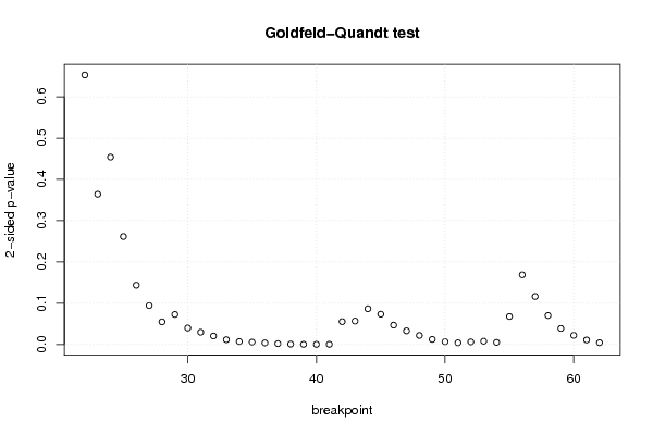
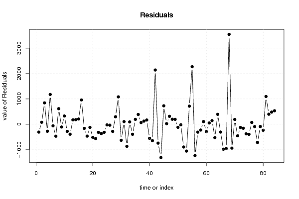
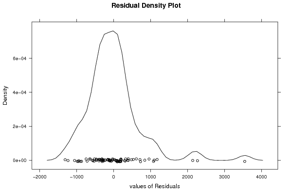
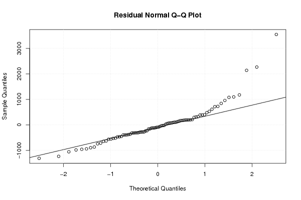
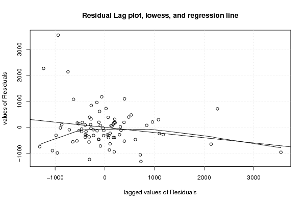
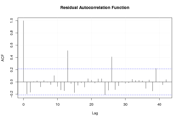
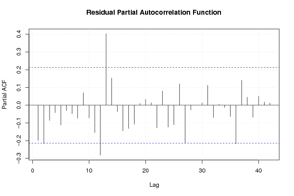
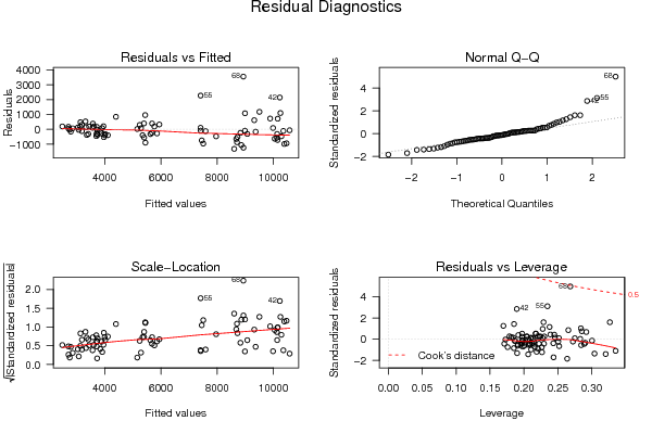
library(lattice) library(lmtest) n25 <- 25 #minimum number of obs. for Goldfeld-Quandt test par1 <- as.numeric(par1) x <- t(y) k <- length(x[1,]) n <- length(x[,1]) x1 <- cbind(x[,par1], x[,1:k!=par1]) mycolnames <- c(colnames(x)[par1], colnames(x)[1:k!=par1]) colnames(x1) <- mycolnames #colnames(x)[par1] x <- x1 if (par3 == 'First Differences'){ x2 <- array(0, dim=c(n-1,k), dimnames=list(1:(n-1), paste('(1-B)',colnames(x),sep=''))) for (i in 1:n-1) { for (j in 1:k) { x2[i,j] <- x[i+1,j] - x[i,j] } } x <- x2 } if (par2 == 'Include Monthly Dummies'){ x2 <- array(0, dim=c(n,11), dimnames=list(1:n, paste('M', seq(1:11), sep =''))) for (i in 1:11){ x2[seq(i,n,12),i] <- 1 } x <- cbind(x, x2) } if (par2 == 'Include Quarterly Dummies'){ x2 <- array(0, dim=c(n,3), dimnames=list(1:n, paste('Q', seq(1:3), sep =''))) for (i in 1:3){ x2[seq(i,n,4),i] <- 1 } x <- cbind(x, x2) } k <- length(x[1,]) if (par3 == 'Linear Trend'){ x <- cbind(x, c(1:n)) colnames(x)[k+1] <- 't' } x k <- length(x[1,]) df <- as.data.frame(x) (mylm <- lm(df)) (mysum <- summary(mylm)) if (n > n25) { kp3 <- k + 3 nmkm3 <- n - k - 3 gqarr <- array(NA, dim=c(nmkm3-kp3+1,3)) numgqtests <- 0 numsignificant1 <- 0 numsignificant5 <- 0 numsignificant10 <- 0 for (mypoint in kp3:nmkm3) { j <- 0 numgqtests <- numgqtests + 1 for (myalt in c('greater', 'two.sided', 'less')) { j <- j + 1 gqarr[mypoint-kp3+1,j] <- gqtest(mylm, point=mypoint, alternative=myalt)$p.value } if (gqarr[mypoint-kp3+1,2] < 0.01) numsignificant1 <- numsignificant1 + 1 if (gqarr[mypoint-kp3+1,2] < 0.05) numsignificant5 <- numsignificant5 + 1 if (gqarr[mypoint-kp3+1,2] < 0.10) numsignificant10 <- numsignificant10 + 1 } gqarr } bitmap(file='test0.png') plot(x[,1], type='l', main='Actuals and Interpolation', ylab='value of Actuals and Interpolation (dots)', xlab='time or index') points(x[,1]-mysum$resid) grid() dev.off() bitmap(file='test1.png') plot(mysum$resid, type='b', pch=19, main='Residuals', ylab='value of Residuals', xlab='time or index') grid() dev.off() bitmap(file='test2.png') hist(mysum$resid, main='Residual Histogram', xlab='values of Residuals') grid() dev.off() bitmap(file='test3.png') densityplot(~mysum$resid,col='black',main='Residual Density Plot', xlab='values of Residuals') dev.off() bitmap(file='test4.png') qqnorm(mysum$resid, main='Residual Normal Q-Q Plot') qqline(mysum$resid) grid() dev.off() (myerror <- as.ts(mysum$resid)) bitmap(file='test5.png') dum <- cbind(lag(myerror,k=1),myerror) dum dum1 <- dum[2:length(myerror),] dum1 z <- as.data.frame(dum1) z plot(z,main=paste('Residual Lag plot, lowess, and regression line'), ylab='values of Residuals', xlab='lagged values of Residuals') lines(lowess(z)) abline(lm(z)) grid() dev.off() bitmap(file='test6.png') acf(mysum$resid, lag.max=length(mysum$resid)/2, main='Residual Autocorrelation Function') grid() dev.off() bitmap(file='test7.png') pacf(mysum$resid, lag.max=length(mysum$resid)/2, main='Residual Partial Autocorrelation Function') grid() dev.off() bitmap(file='test8.png') opar <- par(mfrow = c(2,2), oma = c(0, 0, 1.1, 0)) plot(mylm, las = 1, sub='Residual Diagnostics') par(opar) dev.off() if (n > n25) { bitmap(file='test9.png') plot(kp3:nmkm3,gqarr[,2], main='Goldfeld-Quandt test',ylab='2-sided p-value',xlab='breakpoint') grid() dev.off() } load(file='createtable') a<-table.start() a<-table.row.start(a) a<-table.element(a, 'Multiple Linear Regression - Estimated Regression Equation', 1, TRUE) a<-table.row.end(a) myeq <- colnames(x)[1] myeq <- paste(myeq, '[t] = ', sep='') for (i in 1:k){ if (mysum$coefficients[i,1] > 0) myeq <- paste(myeq, '+', '') myeq <- paste(myeq, mysum$coefficients[i,1], sep=' ') if (rownames(mysum$coefficients)[i] != '(Intercept)') { myeq <- paste(myeq, rownames(mysum$coefficients)[i], sep='') if (rownames(mysum$coefficients)[i] != 't') myeq <- paste(myeq, '[t]', sep='') } } myeq <- paste(myeq, ' + e[t]') a<-table.row.start(a) a<-table.element(a, myeq) a<-table.row.end(a) a<-table.end(a) table.save(a,file='mytable1.tab') a<-table.start() a<-table.row.start(a) a<-table.element(a,hyperlink('http://www.xycoon.com/ols1.htm','Multiple Linear Regression - Ordinary Least Squares',''), 6, TRUE) a<-table.row.end(a) a<-table.row.start(a) a<-table.element(a,'Variable',header=TRUE) a<-table.element(a,'Parameter',header=TRUE) a<-table.element(a,'S.D.',header=TRUE) a<-table.element(a,'T-STAT<br />H0: parameter = 0',header=TRUE) a<-table.element(a,'2-tail p-value',header=TRUE) a<-table.element(a,'1-tail p-value',header=TRUE) a<-table.row.end(a) for (i in 1:k){ a<-table.row.start(a) a<-table.element(a,rownames(mysum$coefficients)[i],header=TRUE) a<-table.element(a,mysum$coefficients[i,1]) a<-table.element(a, round(mysum$coefficients[i,2],6)) a<-table.element(a, round(mysum$coefficients[i,3],4)) a<-table.element(a, round(mysum$coefficients[i,4],6)) a<-table.element(a, round(mysum$coefficients[i,4]/2,6)) a<-table.row.end(a) } a<-table.end(a) table.save(a,file='mytable2.tab') a<-table.start() a<-table.row.start(a) a<-table.element(a, 'Multiple Linear Regression - Regression Statistics', 2, TRUE) a<-table.row.end(a) a<-table.row.start(a) a<-table.element(a, 'Multiple R',1,TRUE) a<-table.element(a, sqrt(mysum$r.squared)) a<-table.row.end(a) a<-table.row.start(a) a<-table.element(a, 'R-squared',1,TRUE) a<-table.element(a, mysum$r.squared) a<-table.row.end(a) a<-table.row.start(a) a<-table.element(a, 'Adjusted R-squared',1,TRUE) a<-table.element(a, mysum$adj.r.squared) a<-table.row.end(a) a<-table.row.start(a) a<-table.element(a, 'F-TEST (value)',1,TRUE) a<-table.element(a, mysum$fstatistic[1]) a<-table.row.end(a) a<-table.row.start(a) a<-table.element(a, 'F-TEST (DF numerator)',1,TRUE) a<-table.element(a, mysum$fstatistic[2]) a<-table.row.end(a) a<-table.row.start(a) a<-table.element(a, 'F-TEST (DF denominator)',1,TRUE) a<-table.element(a, mysum$fstatistic[3]) a<-table.row.end(a) a<-table.row.start(a) a<-table.element(a, 'p-value',1,TRUE) a<-table.element(a, 1-pf(mysum$fstatistic[1],mysum$fstatistic[2],mysum$fstatistic[3])) a<-table.row.end(a) a<-table.row.start(a) a<-table.element(a, 'Multiple Linear Regression - Residual Statistics', 2, TRUE) a<-table.row.end(a) a<-table.row.start(a) a<-table.element(a, 'Residual Standard Deviation',1,TRUE) a<-table.element(a, mysum$sigma) a<-table.row.end(a) a<-table.row.start(a) a<-table.element(a, 'Sum Squared Residuals',1,TRUE) a<-table.element(a, sum(myerror*myerror)) a<-table.row.end(a) a<-table.end(a) table.save(a,file='mytable3.tab') a<-table.start() a<-table.row.start(a) a<-table.element(a, 'Multiple Linear Regression - Actuals, Interpolation, and Residuals', 4, TRUE) a<-table.row.end(a) a<-table.row.start(a) a<-table.element(a, 'Time or Index', 1, TRUE) a<-table.element(a, 'Actuals', 1, TRUE) a<-table.element(a, 'Interpolation<br />Forecast', 1, TRUE) a<-table.element(a, 'Residuals<br />Prediction Error', 1, TRUE) a<-table.row.end(a) for (i in 1:n) { a<-table.row.start(a) a<-table.element(a,i, 1, TRUE) a<-table.element(a,x[i]) a<-table.element(a,x[i]-mysum$resid[i]) a<-table.element(a,mysum$resid[i]) a<-table.row.end(a) } a<-table.end(a) table.save(a,file='mytable4.tab') if (n > n25) { a<-table.start() a<-table.row.start(a) a<-table.element(a,'Goldfeld-Quandt test for Heteroskedasticity',4,TRUE) a<-table.row.end(a) a<-table.row.start(a) a<-table.element(a,'p-values',header=TRUE) a<-table.element(a,'Alternative Hypothesis',3,header=TRUE) a<-table.row.end(a) a<-table.row.start(a) a<-table.element(a,'breakpoint index',header=TRUE) a<-table.element(a,'greater',header=TRUE) a<-table.element(a,'2-sided',header=TRUE) a<-table.element(a,'less',header=TRUE) a<-table.row.end(a) for (mypoint in kp3:nmkm3) { a<-table.row.start(a) a<-table.element(a,mypoint,header=TRUE) a<-table.element(a,gqarr[mypoint-kp3+1,1]) a<-table.element(a,gqarr[mypoint-kp3+1,2]) a<-table.element(a,gqarr[mypoint-kp3+1,3]) a<-table.row.end(a) } a<-table.end(a) table.save(a,file='mytable5.tab') a<-table.start() a<-table.row.start(a) a<-table.element(a,'Meta Analysis of Goldfeld-Quandt test for Heteroskedasticity',4,TRUE) a<-table.row.end(a) a<-table.row.start(a) a<-table.element(a,'Description',header=TRUE) a<-table.element(a,'# significant tests',header=TRUE) a<-table.element(a,'% significant tests',header=TRUE) a<-table.element(a,'OK/NOK',header=TRUE) a<-table.row.end(a) a<-table.row.start(a) a<-table.element(a,'1% type I error level',header=TRUE) a<-table.element(a,numsignificant1) a<-table.element(a,numsignificant1/numgqtests) if (numsignificant1/numgqtests < 0.01) dum <- 'OK' else dum <- 'NOK' a<-table.element(a,dum) a<-table.row.end(a) a<-table.row.start(a) a<-table.element(a,'5% type I error level',header=TRUE) a<-table.element(a,numsignificant5) a<-table.element(a,numsignificant5/numgqtests) if (numsignificant5/numgqtests < 0.05) dum <- 'OK' else dum <- 'NOK' a<-table.element(a,dum) a<-table.row.end(a) a<-table.row.start(a) a<-table.element(a,'10% type I error level',header=TRUE) a<-table.element(a,numsignificant10) a<-table.element(a,numsignificant10/numgqtests) if (numsignificant10/numgqtests < 0.1) dum <- 'OK' else dum <- 'NOK' a<-table.element(a,dum) a<-table.row.end(a) a<-table.end(a) table.save(a,file='mytable6.tab') }

Copyright

This work is licensed under a Creative Commons Attribution-Noncommercial-Share Alike 3.0 License.

Software written by Ed van Stee & Patrick Wessa

Disclaimer

Information provided on this web site is provided "AS IS" without warranty of any kind, either express or implied, including, without limitation, warranties of merchantability, fitness for a particular purpose, and noninfringement. We use reasonable efforts to include accurate and timely information and periodically update the information, and software without notice. However, we make no warranties or representations as to the accuracy or completeness of such information (or software), and we assume no liability or responsibility for errors or omissions in the content of this web site, or any software bugs in online applications. Your use of this web site is AT YOUR OWN RISK. Under no circumstances and under no legal theory shall we be liable to you or any other person for any direct, indirect, special, incidental, exemplary, or consequential damages arising from your access to, or use of, this web site.

Privacy Policy

We may request personal information to be submitted to our servers in order to be able to:

• personalize online software applications according to your needs
• enforce strict security rules with respect to the data that you upload (e.g. statistical data)
• manage user sessions of online applications
• alert you about important changes or upgrades in resources or applications

We NEVER allow other companies to directly offer registered users information about their products and services. Banner references and hyperlinks of third parties NEVER contain any personal data of the visitor.

We do NOT sell, nor transmit by any means, personal information, nor statistical data series uploaded by you to third parties.

We carefully protect your data from loss, misuse, alteration, and destruction. However, at any time, and under any circumstance you are solely responsible for managing your passwords, and keeping them secret.

We store a unique ANONYMOUS USER ID in the form of a small 'Cookie' on your computer. This allows us to track your progress when using this website which is necessary to create state-dependent features. The cookie is used for NO OTHER PURPOSE. At any time you may opt to disallow cookies from this website - this will not affect other features of this website.

We examine cookies that are used by third-parties (banner and online ads) very closely: abuse from third-parties automatically results in termination of the advertising contract without refund. We have very good reason to believe that the cookies that are produced by third parties (banner ads) do NOT cause any privacy or security risk.

FreeStatistics.org is safe. There is no need to download any software to use the applications and services contained in this website. Hence, your system's security is not compromised by their use, and your personal data - other than data you submit in the account application form, and the user-agent information that is transmitted by your browser - is never transmitted to our servers.

As a general rule, we do not log on-line behavior of individuals (other than normal logging of webserver 'hits'). However, in cases of abuse, hacking, unauthorized access, Denial of Service attacks, illegal copying, hotlinking, non-compliance with international webstandards (such as robots.txt), or any other harmful behavior, our system engineers are empowered to log, track, identify, publish, and ban misbehaving individuals - even if this leads to ban entire blocks of IP addresses, or disclosing user's identity.

FreeStatistics.org is powered by