Repository of Reproducible Computations

Free Statistics

of Irreproducible Research!

Author's title

Author

*The author of this computation has been verified*

R Software Module

rwasp_autocorrelation.wasp

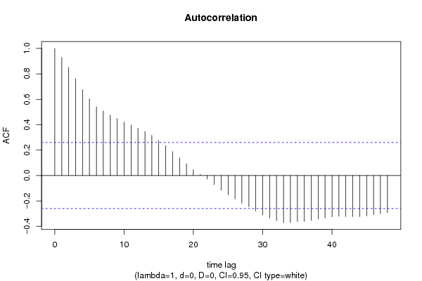
Title produced by software

(Partial) Autocorrelation Function

Date of computation

Tue, 21 Dec 2010 13:33:37 +0000

Cite this page as follows

Statistical Computations at FreeStatistics.org, Office for Research Development and Education, URL https://freestatistics.org/blog/index.php?v=date/2010/Dec/21/t1292938338rvv2yh8ke1ka8ql.htm/, Retrieved Thu, 09 May 2024 14:37:15 +0000

Statistical Computations at FreeStatistics.org, Office for Research Development and Education, URL https://freestatistics.org/blog/index.php?pk=113524, Retrieved Thu, 09 May 2024 14:37:15 +0000

QR Codes:

Paste this QR Code to cite your computation.

Original text written by user:

IsPrivate?

No (this computation is public)

User-defined keywords

Estimated Impact

145

Family? (F = Feedback message, R = changed R code, M = changed R Module, P = changed Parameters, D = changed Data)

-     [Univariate Explorative Data Analysis] [Run Sequence gebo...] [2008-12-12 13:32:37] [76963dc1903f0f612b6153510a3818cf]
- R  D  [Univariate Explorative Data Analysis] [Run Sequence gebo...] [2008-12-17 12:14:40] [76963dc1903f0f612b6153510a3818cf]
-         [Univariate Explorative Data Analysis] [Run Sequence Plot...] [2008-12-22 18:19:51] [1ce0d16c8f4225c977b42c8fa93bc163]
- RMP       [Univariate Data Series] [Identifying Integ...] [2009-11-22 12:08:06] [b98453cac15ba1066b407e146608df68]
- RMP         [(Partial) Autocorrelation Function] [Births] [2010-11-29 09:36:27] [b98453cac15ba1066b407e146608df68]
- R PD          [(Partial) Autocorrelation Function] [WS9 3.1 ACF d=0, D=0] [2010-12-07 10:00:49] [afe9379cca749d06b3d6872e02cc47ed]
-   PD            [(Partial) Autocorrelation Function] [Apple Inc - ACF d...] [2010-12-14 15:49:43] [afe9379cca749d06b3d6872e02cc47ed]
-    D                [(Partial) Autocorrelation Function] [Paper - C&S ACF d...] [2010-12-21 13:33:37] [89d441ae0711e9b79b5d358f420c1317] [Current]
-   P                   [(Partial) Autocorrelation Function] [Paper - C&S ACF d...] [2010-12-21 13:37:41] [18fa53e8b37a5effc0c5f8a5122cdd2d] 

Feedback Forum

Post a new message

Dataseries X:

Download CSV

Histogram

Boxplots

Summary of computational transaction
Raw Input	view raw input (R code)
Raw Output	view raw output of R engine
Computing time	2 seconds
R Server	'RServer@AstonUniversity' @ vre.aston.ac.uk

\begin{tabular}{lllllllll}
\hline
Summary of computational transaction \tabularnewline
Raw Input & view raw input (R code)  \tabularnewline
Raw Output & view raw output of R engine  \tabularnewline
Computing time & 2 seconds \tabularnewline
R Server & 'RServer@AstonUniversity' @ vre.aston.ac.uk \tabularnewline
\hline
\end{tabular}
%Source: https://freestatistics.org/blog/index.php?pk=113524&T=0

[TABLE]
[ROW][C]Summary of computational transaction[/C][/ROW]
[ROW][C]Raw Input[/C][C]view raw input (R code) [/C][/ROW]
[ROW][C]Raw Output[/C][C]view raw output of R engine [/C][/ROW]
[ROW][C]Computing time[/C][C]2 seconds[/C][/ROW]
[ROW][C]R Server[/C][C]'RServer@AstonUniversity' @ vre.aston.ac.uk[/C][/ROW]
[/TABLE]
Source: https://freestatistics.org/blog/index.php?pk=113524&T=0

Globally Unique Identifier (entire table): ba.freestatistics.org/blog/index.php?pk=113524&T=0

As an alternative you can also use a QR Code:

The GUIDs for individual cells are displayed in the table below:

Summary of computational transaction
Raw Input	view raw input (R code)
Raw Output	view raw output of R engine
Computing time	2 seconds
R Server	'RServer@AstonUniversity' @ vre.aston.ac.uk

Autocorrelation Function
Time lag k	ACF(k)	T-STAT	P-value
1	0.929403	7.0168	0
2	0.850169	6.4186	0
3	0.762613	5.7576	0
4	0.676852	5.1101	2e-06
5	0.604076	4.5607	1.4e-05
6	0.541053	4.0849	7e-05
7	0.508074	3.8359	0.000158
8	0.475537	3.5902	0.000344
9	0.447734	3.3803	0.000656
10	0.420405	3.174	0.001212
11	0.397595	3.0018	0.001989
12	0.372927	2.8155	0.003338
13	0.34599	2.6122	0.005741
14	0.315902	2.385	0.010213
15	0.27648	2.0874	0.020668
16	0.235192	1.7757	0.040564
17	0.18909	1.4276	0.079432
18	0.139011	1.0495	0.149187
19	0.092386	0.6975	0.244164
20	0.046199	0.3488	0.364264
21	0.008627	0.0651	0.474148
22	-0.027994	-0.2113	0.416684
23	-0.070835	-0.5348	0.297437
24	-0.114856	-0.8671	0.19475
25	-0.150768	-1.1383	0.129884
26	-0.185031	-1.397	0.083922
27	-0.218025	-1.6461	0.052628
28	-0.245433	-1.853	0.034532
29	-0.278089	-2.0995	0.020105
30	-0.30929	-2.3351	0.011542
31	-0.335523	-2.5331	0.00704
32	-0.354548	-2.6768	0.004845
33	-0.369247	-2.7878	0.0036
34	-0.368292	-2.7805	0.003671
35	-0.361887	-2.7322	0.004181
36	-0.360835	-2.7242	0.004271
37	-0.353764	-2.6709	0.004922
38	-0.34283	-2.5883	0.006108
39	-0.334296	-2.5239	0.007209
40	-0.325421	-2.4569	0.008541
41	-0.320567	-2.4202	0.00936
42	-0.323189	-2.44	0.00891
43	-0.323308	-2.4409	0.00889
44	-0.322837	-2.4374	0.008969
45	-0.316735	-2.3913	0.010056
46	-0.307867	-2.3243	0.011847
47	-0.299093	-2.2581	0.013893
48	-0.290718	-2.1949	0.016131

\begin{tabular}{lllllllll}
\hline
Autocorrelation Function \tabularnewline
Time lag k & ACF(k) & T-STAT & P-value \tabularnewline
1 & 0.929403 & 7.0168 & 0 \tabularnewline
2 & 0.850169 & 6.4186 & 0 \tabularnewline
3 & 0.762613 & 5.7576 & 0 \tabularnewline
4 & 0.676852 & 5.1101 & 2e-06 \tabularnewline
5 & 0.604076 & 4.5607 & 1.4e-05 \tabularnewline
6 & 0.541053 & 4.0849 & 7e-05 \tabularnewline
7 & 0.508074 & 3.8359 & 0.000158 \tabularnewline
8 & 0.475537 & 3.5902 & 0.000344 \tabularnewline
9 & 0.447734 & 3.3803 & 0.000656 \tabularnewline
10 & 0.420405 & 3.174 & 0.001212 \tabularnewline
11 & 0.397595 & 3.0018 & 0.001989 \tabularnewline
12 & 0.372927 & 2.8155 & 0.003338 \tabularnewline
13 & 0.34599 & 2.6122 & 0.005741 \tabularnewline
14 & 0.315902 & 2.385 & 0.010213 \tabularnewline
15 & 0.27648 & 2.0874 & 0.020668 \tabularnewline
16 & 0.235192 & 1.7757 & 0.040564 \tabularnewline
17 & 0.18909 & 1.4276 & 0.079432 \tabularnewline
18 & 0.139011 & 1.0495 & 0.149187 \tabularnewline
19 & 0.092386 & 0.6975 & 0.244164 \tabularnewline
20 & 0.046199 & 0.3488 & 0.364264 \tabularnewline
21 & 0.008627 & 0.0651 & 0.474148 \tabularnewline
22 & -0.027994 & -0.2113 & 0.416684 \tabularnewline
23 & -0.070835 & -0.5348 & 0.297437 \tabularnewline
24 & -0.114856 & -0.8671 & 0.19475 \tabularnewline
25 & -0.150768 & -1.1383 & 0.129884 \tabularnewline
26 & -0.185031 & -1.397 & 0.083922 \tabularnewline
27 & -0.218025 & -1.6461 & 0.052628 \tabularnewline
28 & -0.245433 & -1.853 & 0.034532 \tabularnewline
29 & -0.278089 & -2.0995 & 0.020105 \tabularnewline
30 & -0.30929 & -2.3351 & 0.011542 \tabularnewline
31 & -0.335523 & -2.5331 & 0.00704 \tabularnewline
32 & -0.354548 & -2.6768 & 0.004845 \tabularnewline
33 & -0.369247 & -2.7878 & 0.0036 \tabularnewline
34 & -0.368292 & -2.7805 & 0.003671 \tabularnewline
35 & -0.361887 & -2.7322 & 0.004181 \tabularnewline
36 & -0.360835 & -2.7242 & 0.004271 \tabularnewline
37 & -0.353764 & -2.6709 & 0.004922 \tabularnewline
38 & -0.34283 & -2.5883 & 0.006108 \tabularnewline
39 & -0.334296 & -2.5239 & 0.007209 \tabularnewline
40 & -0.325421 & -2.4569 & 0.008541 \tabularnewline
41 & -0.320567 & -2.4202 & 0.00936 \tabularnewline
42 & -0.323189 & -2.44 & 0.00891 \tabularnewline
43 & -0.323308 & -2.4409 & 0.00889 \tabularnewline
44 & -0.322837 & -2.4374 & 0.008969 \tabularnewline
45 & -0.316735 & -2.3913 & 0.010056 \tabularnewline
46 & -0.307867 & -2.3243 & 0.011847 \tabularnewline
47 & -0.299093 & -2.2581 & 0.013893 \tabularnewline
48 & -0.290718 & -2.1949 & 0.016131 \tabularnewline
\hline
\end{tabular}
%Source: https://freestatistics.org/blog/index.php?pk=113524&T=1

[TABLE]
[ROW][C]Autocorrelation Function[/C][/ROW]
[ROW][C]Time lag k[/C][C]ACF(k)[/C][C]T-STAT[/C][C]P-value[/C][/ROW]
[ROW][C]1[/C][C]0.929403[/C][C]7.0168[/C][C]0[/C][/ROW]
[ROW][C]2[/C][C]0.850169[/C][C]6.4186[/C][C]0[/C][/ROW]
[ROW][C]3[/C][C]0.762613[/C][C]5.7576[/C][C]0[/C][/ROW]
[ROW][C]4[/C][C]0.676852[/C][C]5.1101[/C][C]2e-06[/C][/ROW]
[ROW][C]5[/C][C]0.604076[/C][C]4.5607[/C][C]1.4e-05[/C][/ROW]
[ROW][C]6[/C][C]0.541053[/C][C]4.0849[/C][C]7e-05[/C][/ROW]
[ROW][C]7[/C][C]0.508074[/C][C]3.8359[/C][C]0.000158[/C][/ROW]
[ROW][C]8[/C][C]0.475537[/C][C]3.5902[/C][C]0.000344[/C][/ROW]
[ROW][C]9[/C][C]0.447734[/C][C]3.3803[/C][C]0.000656[/C][/ROW]
[ROW][C]10[/C][C]0.420405[/C][C]3.174[/C][C]0.001212[/C][/ROW]
[ROW][C]11[/C][C]0.397595[/C][C]3.0018[/C][C]0.001989[/C][/ROW]
[ROW][C]12[/C][C]0.372927[/C][C]2.8155[/C][C]0.003338[/C][/ROW]
[ROW][C]13[/C][C]0.34599[/C][C]2.6122[/C][C]0.005741[/C][/ROW]
[ROW][C]14[/C][C]0.315902[/C][C]2.385[/C][C]0.010213[/C][/ROW]
[ROW][C]15[/C][C]0.27648[/C][C]2.0874[/C][C]0.020668[/C][/ROW]
[ROW][C]16[/C][C]0.235192[/C][C]1.7757[/C][C]0.040564[/C][/ROW]
[ROW][C]17[/C][C]0.18909[/C][C]1.4276[/C][C]0.079432[/C][/ROW]
[ROW][C]18[/C][C]0.139011[/C][C]1.0495[/C][C]0.149187[/C][/ROW]
[ROW][C]19[/C][C]0.092386[/C][C]0.6975[/C][C]0.244164[/C][/ROW]
[ROW][C]20[/C][C]0.046199[/C][C]0.3488[/C][C]0.364264[/C][/ROW]
[ROW][C]21[/C][C]0.008627[/C][C]0.0651[/C][C]0.474148[/C][/ROW]
[ROW][C]22[/C][C]-0.027994[/C][C]-0.2113[/C][C]0.416684[/C][/ROW]
[ROW][C]23[/C][C]-0.070835[/C][C]-0.5348[/C][C]0.297437[/C][/ROW]
[ROW][C]24[/C][C]-0.114856[/C][C]-0.8671[/C][C]0.19475[/C][/ROW]
[ROW][C]25[/C][C]-0.150768[/C][C]-1.1383[/C][C]0.129884[/C][/ROW]
[ROW][C]26[/C][C]-0.185031[/C][C]-1.397[/C][C]0.083922[/C][/ROW]
[ROW][C]27[/C][C]-0.218025[/C][C]-1.6461[/C][C]0.052628[/C][/ROW]
[ROW][C]28[/C][C]-0.245433[/C][C]-1.853[/C][C]0.034532[/C][/ROW]
[ROW][C]29[/C][C]-0.278089[/C][C]-2.0995[/C][C]0.020105[/C][/ROW]
[ROW][C]30[/C][C]-0.30929[/C][C]-2.3351[/C][C]0.011542[/C][/ROW]
[ROW][C]31[/C][C]-0.335523[/C][C]-2.5331[/C][C]0.00704[/C][/ROW]
[ROW][C]32[/C][C]-0.354548[/C][C]-2.6768[/C][C]0.004845[/C][/ROW]
[ROW][C]33[/C][C]-0.369247[/C][C]-2.7878[/C][C]0.0036[/C][/ROW]
[ROW][C]34[/C][C]-0.368292[/C][C]-2.7805[/C][C]0.003671[/C][/ROW]
[ROW][C]35[/C][C]-0.361887[/C][C]-2.7322[/C][C]0.004181[/C][/ROW]
[ROW][C]36[/C][C]-0.360835[/C][C]-2.7242[/C][C]0.004271[/C][/ROW]
[ROW][C]37[/C][C]-0.353764[/C][C]-2.6709[/C][C]0.004922[/C][/ROW]
[ROW][C]38[/C][C]-0.34283[/C][C]-2.5883[/C][C]0.006108[/C][/ROW]
[ROW][C]39[/C][C]-0.334296[/C][C]-2.5239[/C][C]0.007209[/C][/ROW]
[ROW][C]40[/C][C]-0.325421[/C][C]-2.4569[/C][C]0.008541[/C][/ROW]
[ROW][C]41[/C][C]-0.320567[/C][C]-2.4202[/C][C]0.00936[/C][/ROW]
[ROW][C]42[/C][C]-0.323189[/C][C]-2.44[/C][C]0.00891[/C][/ROW]
[ROW][C]43[/C][C]-0.323308[/C][C]-2.4409[/C][C]0.00889[/C][/ROW]
[ROW][C]44[/C][C]-0.322837[/C][C]-2.4374[/C][C]0.008969[/C][/ROW]
[ROW][C]45[/C][C]-0.316735[/C][C]-2.3913[/C][C]0.010056[/C][/ROW]
[ROW][C]46[/C][C]-0.307867[/C][C]-2.3243[/C][C]0.011847[/C][/ROW]
[ROW][C]47[/C][C]-0.299093[/C][C]-2.2581[/C][C]0.013893[/C][/ROW]
[ROW][C]48[/C][C]-0.290718[/C][C]-2.1949[/C][C]0.016131[/C][/ROW]
[/TABLE]
Source: https://freestatistics.org/blog/index.php?pk=113524&T=1

Globally Unique Identifier (entire table): ba.freestatistics.org/blog/index.php?pk=113524&T=1

As an alternative you can also use a QR Code:

The GUIDs for individual cells are displayed in the table below:

Autocorrelation Function
Time lag k	ACF(k)	T-STAT	P-value
1	0.929403	7.0168	0
2	0.850169	6.4186	0
3	0.762613	5.7576	0
4	0.676852	5.1101	2e-06
5	0.604076	4.5607	1.4e-05
6	0.541053	4.0849	7e-05
7	0.508074	3.8359	0.000158
8	0.475537	3.5902	0.000344
9	0.447734	3.3803	0.000656
10	0.420405	3.174	0.001212
11	0.397595	3.0018	0.001989
12	0.372927	2.8155	0.003338
13	0.34599	2.6122	0.005741
14	0.315902	2.385	0.010213
15	0.27648	2.0874	0.020668
16	0.235192	1.7757	0.040564
17	0.18909	1.4276	0.079432
18	0.139011	1.0495	0.149187
19	0.092386	0.6975	0.244164
20	0.046199	0.3488	0.364264
21	0.008627	0.0651	0.474148
22	-0.027994	-0.2113	0.416684
23	-0.070835	-0.5348	0.297437
24	-0.114856	-0.8671	0.19475
25	-0.150768	-1.1383	0.129884
26	-0.185031	-1.397	0.083922
27	-0.218025	-1.6461	0.052628
28	-0.245433	-1.853	0.034532
29	-0.278089	-2.0995	0.020105
30	-0.30929	-2.3351	0.011542
31	-0.335523	-2.5331	0.00704
32	-0.354548	-2.6768	0.004845
33	-0.369247	-2.7878	0.0036
34	-0.368292	-2.7805	0.003671
35	-0.361887	-2.7322	0.004181
36	-0.360835	-2.7242	0.004271
37	-0.353764	-2.6709	0.004922
38	-0.34283	-2.5883	0.006108
39	-0.334296	-2.5239	0.007209
40	-0.325421	-2.4569	0.008541
41	-0.320567	-2.4202	0.00936
42	-0.323189	-2.44	0.00891
43	-0.323308	-2.4409	0.00889
44	-0.322837	-2.4374	0.008969
45	-0.316735	-2.3913	0.010056
46	-0.307867	-2.3243	0.011847
47	-0.299093	-2.2581	0.013893
48	-0.290718	-2.1949	0.016131

Partial Autocorrelation Function
Time lag k	PACF(k)	T-STAT	P-value
1	0.929403	7.0168	0
2	-0.1	-0.755	0.226684
3	-0.10094	-0.7621	0.224577
4	-0.030005	-0.2265	0.410799
5	0.047642	0.3597	0.360204
6	0.015658	0.1182	0.453157
7	0.165781	1.2516	0.10791
8	-0.051352	-0.3877	0.34984
9	-0.006149	-0.0464	0.481568
10	-0.011592	-0.0875	0.465282
11	0.043396	0.3276	0.372195
12	-0.021552	-0.1627	0.43566
13	0.001889	0.0143	0.494337
14	-0.048625	-0.3671	0.357449
15	-0.075302	-0.5685	0.285958
16	-0.02948	-0.2226	0.412332
17	-0.040522	-0.3059	0.380385
18	-0.069936	-0.528	0.299772
19	-0.013965	-0.1054	0.4582
20	-0.051858	-0.3915	0.348436
21	-0.002112	-0.0159	0.493665
22	-0.046549	-0.3514	0.363279
23	-0.106184	-0.8017	0.213037
24	-0.067702	-0.5111	0.305613
25	0.031532	0.2381	0.406345
26	-0.040735	-0.3075	0.379776
27	-0.037099	-0.2801	0.390209
28	-0.017913	-0.1352	0.44645
29	-0.102311	-0.7724	0.221525
30	-0.038089	-0.2876	0.387361
31	0.02996	0.2262	0.41093
32	0.009379	0.0708	0.471897
33	-0.02656	-0.2005	0.420892
34	0.088182	0.6658	0.254126
35	-0.013285	-0.1003	0.460228
36	-0.066359	-0.501	0.309149
37	0.060033	0.4532	0.326048
38	0.046756	0.353	0.362696
39	-0.034199	-0.2582	0.398592
40	0.038413	0.29	0.386431
41	-0.037547	-0.2835	0.388922
42	-0.093382	-0.705	0.241835
43	0.041158	0.3107	0.378569
44	0.008507	0.0642	0.474508
45	0.004061	0.0307	0.487825
46	0.003125	0.0236	0.490629
47	-0.055542	-0.4193	0.338276
48	-0.074295	-0.5609	0.288526

\begin{tabular}{lllllllll}
\hline
Partial Autocorrelation Function \tabularnewline
Time lag k & PACF(k) & T-STAT & P-value \tabularnewline
1 & 0.929403 & 7.0168 & 0 \tabularnewline
2 & -0.1 & -0.755 & 0.226684 \tabularnewline
3 & -0.10094 & -0.7621 & 0.224577 \tabularnewline
4 & -0.030005 & -0.2265 & 0.410799 \tabularnewline
5 & 0.047642 & 0.3597 & 0.360204 \tabularnewline
6 & 0.015658 & 0.1182 & 0.453157 \tabularnewline
7 & 0.165781 & 1.2516 & 0.10791 \tabularnewline
8 & -0.051352 & -0.3877 & 0.34984 \tabularnewline
9 & -0.006149 & -0.0464 & 0.481568 \tabularnewline
10 & -0.011592 & -0.0875 & 0.465282 \tabularnewline
11 & 0.043396 & 0.3276 & 0.372195 \tabularnewline
12 & -0.021552 & -0.1627 & 0.43566 \tabularnewline
13 & 0.001889 & 0.0143 & 0.494337 \tabularnewline
14 & -0.048625 & -0.3671 & 0.357449 \tabularnewline
15 & -0.075302 & -0.5685 & 0.285958 \tabularnewline
16 & -0.02948 & -0.2226 & 0.412332 \tabularnewline
17 & -0.040522 & -0.3059 & 0.380385 \tabularnewline
18 & -0.069936 & -0.528 & 0.299772 \tabularnewline
19 & -0.013965 & -0.1054 & 0.4582 \tabularnewline
20 & -0.051858 & -0.3915 & 0.348436 \tabularnewline
21 & -0.002112 & -0.0159 & 0.493665 \tabularnewline
22 & -0.046549 & -0.3514 & 0.363279 \tabularnewline
23 & -0.106184 & -0.8017 & 0.213037 \tabularnewline
24 & -0.067702 & -0.5111 & 0.305613 \tabularnewline
25 & 0.031532 & 0.2381 & 0.406345 \tabularnewline
26 & -0.040735 & -0.3075 & 0.379776 \tabularnewline
27 & -0.037099 & -0.2801 & 0.390209 \tabularnewline
28 & -0.017913 & -0.1352 & 0.44645 \tabularnewline
29 & -0.102311 & -0.7724 & 0.221525 \tabularnewline
30 & -0.038089 & -0.2876 & 0.387361 \tabularnewline
31 & 0.02996 & 0.2262 & 0.41093 \tabularnewline
32 & 0.009379 & 0.0708 & 0.471897 \tabularnewline
33 & -0.02656 & -0.2005 & 0.420892 \tabularnewline
34 & 0.088182 & 0.6658 & 0.254126 \tabularnewline
35 & -0.013285 & -0.1003 & 0.460228 \tabularnewline
36 & -0.066359 & -0.501 & 0.309149 \tabularnewline
37 & 0.060033 & 0.4532 & 0.326048 \tabularnewline
38 & 0.046756 & 0.353 & 0.362696 \tabularnewline
39 & -0.034199 & -0.2582 & 0.398592 \tabularnewline
40 & 0.038413 & 0.29 & 0.386431 \tabularnewline
41 & -0.037547 & -0.2835 & 0.388922 \tabularnewline
42 & -0.093382 & -0.705 & 0.241835 \tabularnewline
43 & 0.041158 & 0.3107 & 0.378569 \tabularnewline
44 & 0.008507 & 0.0642 & 0.474508 \tabularnewline
45 & 0.004061 & 0.0307 & 0.487825 \tabularnewline
46 & 0.003125 & 0.0236 & 0.490629 \tabularnewline
47 & -0.055542 & -0.4193 & 0.338276 \tabularnewline
48 & -0.074295 & -0.5609 & 0.288526 \tabularnewline
\hline
\end{tabular}
%Source: https://freestatistics.org/blog/index.php?pk=113524&T=2

[TABLE]
[ROW][C]Partial Autocorrelation Function[/C][/ROW]
[ROW][C]Time lag k[/C][C]PACF(k)[/C][C]T-STAT[/C][C]P-value[/C][/ROW]
[ROW][C]1[/C][C]0.929403[/C][C]7.0168[/C][C]0[/C][/ROW]
[ROW][C]2[/C][C]-0.1[/C][C]-0.755[/C][C]0.226684[/C][/ROW]
[ROW][C]3[/C][C]-0.10094[/C][C]-0.7621[/C][C]0.224577[/C][/ROW]
[ROW][C]4[/C][C]-0.030005[/C][C]-0.2265[/C][C]0.410799[/C][/ROW]
[ROW][C]5[/C][C]0.047642[/C][C]0.3597[/C][C]0.360204[/C][/ROW]
[ROW][C]6[/C][C]0.015658[/C][C]0.1182[/C][C]0.453157[/C][/ROW]
[ROW][C]7[/C][C]0.165781[/C][C]1.2516[/C][C]0.10791[/C][/ROW]
[ROW][C]8[/C][C]-0.051352[/C][C]-0.3877[/C][C]0.34984[/C][/ROW]
[ROW][C]9[/C][C]-0.006149[/C][C]-0.0464[/C][C]0.481568[/C][/ROW]
[ROW][C]10[/C][C]-0.011592[/C][C]-0.0875[/C][C]0.465282[/C][/ROW]
[ROW][C]11[/C][C]0.043396[/C][C]0.3276[/C][C]0.372195[/C][/ROW]
[ROW][C]12[/C][C]-0.021552[/C][C]-0.1627[/C][C]0.43566[/C][/ROW]
[ROW][C]13[/C][C]0.001889[/C][C]0.0143[/C][C]0.494337[/C][/ROW]
[ROW][C]14[/C][C]-0.048625[/C][C]-0.3671[/C][C]0.357449[/C][/ROW]
[ROW][C]15[/C][C]-0.075302[/C][C]-0.5685[/C][C]0.285958[/C][/ROW]
[ROW][C]16[/C][C]-0.02948[/C][C]-0.2226[/C][C]0.412332[/C][/ROW]
[ROW][C]17[/C][C]-0.040522[/C][C]-0.3059[/C][C]0.380385[/C][/ROW]
[ROW][C]18[/C][C]-0.069936[/C][C]-0.528[/C][C]0.299772[/C][/ROW]
[ROW][C]19[/C][C]-0.013965[/C][C]-0.1054[/C][C]0.4582[/C][/ROW]
[ROW][C]20[/C][C]-0.051858[/C][C]-0.3915[/C][C]0.348436[/C][/ROW]
[ROW][C]21[/C][C]-0.002112[/C][C]-0.0159[/C][C]0.493665[/C][/ROW]
[ROW][C]22[/C][C]-0.046549[/C][C]-0.3514[/C][C]0.363279[/C][/ROW]
[ROW][C]23[/C][C]-0.106184[/C][C]-0.8017[/C][C]0.213037[/C][/ROW]
[ROW][C]24[/C][C]-0.067702[/C][C]-0.5111[/C][C]0.305613[/C][/ROW]
[ROW][C]25[/C][C]0.031532[/C][C]0.2381[/C][C]0.406345[/C][/ROW]
[ROW][C]26[/C][C]-0.040735[/C][C]-0.3075[/C][C]0.379776[/C][/ROW]
[ROW][C]27[/C][C]-0.037099[/C][C]-0.2801[/C][C]0.390209[/C][/ROW]
[ROW][C]28[/C][C]-0.017913[/C][C]-0.1352[/C][C]0.44645[/C][/ROW]
[ROW][C]29[/C][C]-0.102311[/C][C]-0.7724[/C][C]0.221525[/C][/ROW]
[ROW][C]30[/C][C]-0.038089[/C][C]-0.2876[/C][C]0.387361[/C][/ROW]
[ROW][C]31[/C][C]0.02996[/C][C]0.2262[/C][C]0.41093[/C][/ROW]
[ROW][C]32[/C][C]0.009379[/C][C]0.0708[/C][C]0.471897[/C][/ROW]
[ROW][C]33[/C][C]-0.02656[/C][C]-0.2005[/C][C]0.420892[/C][/ROW]
[ROW][C]34[/C][C]0.088182[/C][C]0.6658[/C][C]0.254126[/C][/ROW]
[ROW][C]35[/C][C]-0.013285[/C][C]-0.1003[/C][C]0.460228[/C][/ROW]
[ROW][C]36[/C][C]-0.066359[/C][C]-0.501[/C][C]0.309149[/C][/ROW]
[ROW][C]37[/C][C]0.060033[/C][C]0.4532[/C][C]0.326048[/C][/ROW]
[ROW][C]38[/C][C]0.046756[/C][C]0.353[/C][C]0.362696[/C][/ROW]
[ROW][C]39[/C][C]-0.034199[/C][C]-0.2582[/C][C]0.398592[/C][/ROW]
[ROW][C]40[/C][C]0.038413[/C][C]0.29[/C][C]0.386431[/C][/ROW]
[ROW][C]41[/C][C]-0.037547[/C][C]-0.2835[/C][C]0.388922[/C][/ROW]
[ROW][C]42[/C][C]-0.093382[/C][C]-0.705[/C][C]0.241835[/C][/ROW]
[ROW][C]43[/C][C]0.041158[/C][C]0.3107[/C][C]0.378569[/C][/ROW]
[ROW][C]44[/C][C]0.008507[/C][C]0.0642[/C][C]0.474508[/C][/ROW]
[ROW][C]45[/C][C]0.004061[/C][C]0.0307[/C][C]0.487825[/C][/ROW]
[ROW][C]46[/C][C]0.003125[/C][C]0.0236[/C][C]0.490629[/C][/ROW]
[ROW][C]47[/C][C]-0.055542[/C][C]-0.4193[/C][C]0.338276[/C][/ROW]
[ROW][C]48[/C][C]-0.074295[/C][C]-0.5609[/C][C]0.288526[/C][/ROW]
[/TABLE]
Source: https://freestatistics.org/blog/index.php?pk=113524&T=2

Globally Unique Identifier (entire table): ba.freestatistics.org/blog/index.php?pk=113524&T=2

As an alternative you can also use a QR Code:

The GUIDs for individual cells are displayed in the table below:

Partial Autocorrelation Function
Time lag k	PACF(k)	T-STAT	P-value
1	0.929403	7.0168	0
2	-0.1	-0.755	0.226684
3	-0.10094	-0.7621	0.224577
4	-0.030005	-0.2265	0.410799
5	0.047642	0.3597	0.360204
6	0.015658	0.1182	0.453157
7	0.165781	1.2516	0.10791
8	-0.051352	-0.3877	0.34984
9	-0.006149	-0.0464	0.481568
10	-0.011592	-0.0875	0.465282
11	0.043396	0.3276	0.372195
12	-0.021552	-0.1627	0.43566
13	0.001889	0.0143	0.494337
14	-0.048625	-0.3671	0.357449
15	-0.075302	-0.5685	0.285958
16	-0.02948	-0.2226	0.412332
17	-0.040522	-0.3059	0.380385
18	-0.069936	-0.528	0.299772
19	-0.013965	-0.1054	0.4582
20	-0.051858	-0.3915	0.348436
21	-0.002112	-0.0159	0.493665
22	-0.046549	-0.3514	0.363279
23	-0.106184	-0.8017	0.213037
24	-0.067702	-0.5111	0.305613
25	0.031532	0.2381	0.406345
26	-0.040735	-0.3075	0.379776
27	-0.037099	-0.2801	0.390209
28	-0.017913	-0.1352	0.44645
29	-0.102311	-0.7724	0.221525
30	-0.038089	-0.2876	0.387361
31	0.02996	0.2262	0.41093
32	0.009379	0.0708	0.471897
33	-0.02656	-0.2005	0.420892
34	0.088182	0.6658	0.254126
35	-0.013285	-0.1003	0.460228
36	-0.066359	-0.501	0.309149
37	0.060033	0.4532	0.326048
38	0.046756	0.353	0.362696
39	-0.034199	-0.2582	0.398592
40	0.038413	0.29	0.386431
41	-0.037547	-0.2835	0.388922
42	-0.093382	-0.705	0.241835
43	0.041158	0.3107	0.378569
44	0.008507	0.0642	0.474508
45	0.004061	0.0307	0.487825
46	0.003125	0.0236	0.490629
47	-0.055542	-0.4193	0.338276
48	-0.074295	-0.5609	0.288526

Figure 1

PNG link

Postscript link

PDF link

Figure 2

PNG link

Postscript link

PDF link

Parameters (Session):

par1 = 48 ; par2 = 1 ; par3 = 0 ; par4 = 0 ; par5 = 12 ; par6 = White Noise ; par7 = 0.95 ;

Parameters (R input):

par1 = 48 ; par2 = 1 ; par3 = 0 ; par4 = 0 ; par5 = 12 ; par6 = White Noise ; par7 = 0.95 ; par8 = ;

R code (references can be found in the software module):

if (par1 == 'Default') {
par1 = 10*log10(length(x))
} else {
par1 <- as.numeric(par1)
}
par2 <- as.numeric(par2)
par3 <- as.numeric(par3)
par4 <- as.numeric(par4)
par5 <- as.numeric(par5)
if (par6 == 'White Noise') par6 <- 'white' else par6 <- 'ma'
par7 <- as.numeric(par7)
if (par2 == 0) {
x <- log(x)
} else {
x <- (x ^ par2 - 1) / par2
}
if (par3 > 0) x <- diff(x,lag=1,difference=par3)
if (par4 > 0) x <- diff(x,lag=par5,difference=par4)
bitmap(file='pic1.png')
racf <- acf(x, par1, main='Autocorrelation', xlab='time lag', ylab='ACF', ci.type=par6, ci=par7, sub=paste('(lambda=',par2,', d=',par3,', D=',par4,', CI=', par7, ', CI type=',par6,')',sep=''))
dev.off()
bitmap(file='pic2.png')
rpacf <- pacf(x,par1,main='Partial Autocorrelation',xlab='lags',ylab='PACF')
dev.off()
(myacf <- c(racf$acf))
(mypacf <- c(rpacf$acf))
lengthx <- length(x)
sqrtn <- sqrt(lengthx)
load(file='createtable')
a<-table.start()
a<-table.row.start(a)
a<-table.element(a,'Autocorrelation Function',4,TRUE)
a<-table.row.end(a)
a<-table.row.start(a)
a<-table.element(a,'Time lag k',header=TRUE)
a<-table.element(a,hyperlink('basics.htm','ACF(k)','click here for more information about the Autocorrelation Function'),header=TRUE)
a<-table.element(a,'T-STAT',header=TRUE)
a<-table.element(a,'P-value',header=TRUE)
a<-table.row.end(a)
for (i in 2:(par1+1)) {
a<-table.row.start(a)
a<-table.element(a,i-1,header=TRUE)
a<-table.element(a,round(myacf[i],6))
mytstat <- myacf[i]*sqrtn
a<-table.element(a,round(mytstat,4))
a<-table.element(a,round(1-pt(abs(mytstat),lengthx),6))
a<-table.row.end(a)
}
a<-table.end(a)
table.save(a,file='mytable.tab')
a<-table.start()
a<-table.row.start(a)
a<-table.element(a,'Partial Autocorrelation Function',4,TRUE)
a<-table.row.end(a)
a<-table.row.start(a)
a<-table.element(a,'Time lag k',header=TRUE)
a<-table.element(a,hyperlink('basics.htm','PACF(k)','click here for more information about the Partial Autocorrelation Function'),header=TRUE)
a<-table.element(a,'T-STAT',header=TRUE)
a<-table.element(a,'P-value',header=TRUE)
a<-table.row.end(a)
for (i in 1:par1) {
a<-table.row.start(a)
a<-table.element(a,i,header=TRUE)
a<-table.element(a,round(mypacf[i],6))
mytstat <- mypacf[i]*sqrtn
a<-table.element(a,round(mytstat,4))
a<-table.element(a,round(1-pt(abs(mytstat),lengthx),6))
a<-table.row.end(a)
}
a<-table.end(a)
table.save(a,file='mytable1.tab')

Free Statistics

Description of Statistical Computation

Tree of Dependent Computations

Dataset

Tables (Output of Computation)

Figures (Output of Computation)

Input Parameters & R Code