Repository of Reproducible Computations

Free Statistics

of Irreproducible Research!

Author's title

Author

*The author of this computation has been verified*

R Software Module

rwasp_autocorrelation.wasp

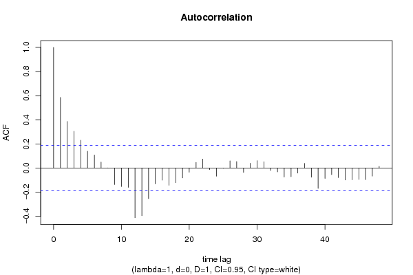
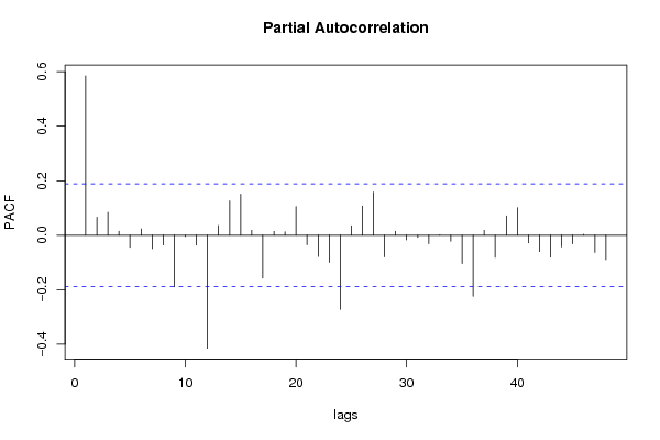
Title produced by software

(Partial) Autocorrelation Function

Date of computation

Tue, 21 Dec 2010 12:22:09 +0000

Cite this page as follows

Statistical Computations at FreeStatistics.org, Office for Research Development and Education, URL https://freestatistics.org/blog/index.php?v=date/2010/Dec/21/t1292934019y98tyodpxr4p5vo.htm/, Retrieved Thu, 09 May 2024 04:41:16 +0000

Statistical Computations at FreeStatistics.org, Office for Research Development and Education, URL https://freestatistics.org/blog/index.php?pk=113374, Retrieved Thu, 09 May 2024 04:41:16 +0000

QR Codes:

Paste this QR Code to cite your computation.

Original text written by user:

IsPrivate?

No (this computation is public)

User-defined keywords

Estimated Impact

171

Family? (F = Feedback message, R = changed R code, M = changed R Module, P = changed Parameters, D = changed Data)

-     [Univariate Data Series] [data set] [2008-12-01 19:54:57] [b98453cac15ba1066b407e146608df68]
- RMP   [(Partial) Autocorrelation Function] [Unemployment] [2010-11-29 09:05:21] [b98453cac15ba1066b407e146608df68]
-    D    [(Partial) Autocorrelation Function] [Workshop 9] [2010-12-03 10:43:29] [39c51da0be01189e8a44eb69e891b7a1]
-   P       [(Partial) Autocorrelation Function] [Workshop 9] [2010-12-03 10:48:00] [39c51da0be01189e8a44eb69e891b7a1]
-   P         [(Partial) Autocorrelation Function] [Workshop 9] [2010-12-03 12:19:31] [39c51da0be01189e8a44eb69e891b7a1]
-    D            [(Partial) Autocorrelation Function] [Autocorrelation A...] [2010-12-21 12:22:09] [2e49bff66bb3e1f5d7fa8957e12fbb12] [Current]
-   P               [(Partial) Autocorrelation Function] [Autocorrelation A...] [2010-12-21 13:51:25] [f9eaed74daea918f73b9f505c5b1f19e] 
-   P               [(Partial) Autocorrelation Function] [Autocorrelation A...] [2010-12-21 14:56:54] [f9eaed74daea918f73b9f505c5b1f19e] 

Feedback Forum

Post a new message

Dataseries X:

Download CSV

Histogram

Boxplots

Summary of computational transaction
Raw Input	view raw input (R code)
Raw Output	view raw output of R engine
Computing time	2 seconds
R Server	'Sir Ronald Aylmer Fisher' @ 193.190.124.24

\begin{tabular}{lllllllll}
\hline
Summary of computational transaction \tabularnewline
Raw Input & view raw input (R code)  \tabularnewline
Raw Output & view raw output of R engine  \tabularnewline
Computing time & 2 seconds \tabularnewline
R Server & 'Sir Ronald Aylmer Fisher' @ 193.190.124.24 \tabularnewline
\hline
\end{tabular}
%Source: https://freestatistics.org/blog/index.php?pk=113374&T=0

[TABLE]
[ROW][C]Summary of computational transaction[/C][/ROW]
[ROW][C]Raw Input[/C][C]view raw input (R code) [/C][/ROW]
[ROW][C]Raw Output[/C][C]view raw output of R engine [/C][/ROW]
[ROW][C]Computing time[/C][C]2 seconds[/C][/ROW]
[ROW][C]R Server[/C][C]'Sir Ronald Aylmer Fisher' @ 193.190.124.24[/C][/ROW]
[/TABLE]
Source: https://freestatistics.org/blog/index.php?pk=113374&T=0

Globally Unique Identifier (entire table): ba.freestatistics.org/blog/index.php?pk=113374&T=0

As an alternative you can also use a QR Code:

The GUIDs for individual cells are displayed in the table below:

Summary of computational transaction
Raw Input	view raw input (R code)
Raw Output	view raw output of R engine
Computing time	2 seconds
R Server	'Sir Ronald Aylmer Fisher' @ 193.190.124.24

Autocorrelation Function
Time lag k	ACF(k)	T-STAT	P-value
1	0.584722	6.0766	0
2	0.385123	4.0023	5.8e-05
3	0.30388	3.158	0.00103
4	0.230334	2.3937	0.009202
5	0.139107	1.4456	0.075586
6	0.107584	1.118	0.133015
7	0.049605	0.5155	0.303626
8	-0.000588	-0.0061	0.497568
9	-0.137252	-1.4264	0.078324
10	-0.153305	-1.5932	0.057019
11	-0.161045	-1.6736	0.048549
12	-0.412335	-4.2851	2e-05
13	-0.396388	-4.1194	3.7e-05
14	-0.253967	-2.6393	0.004768
15	-0.131527	-1.3669	0.087253
16	-0.101399	-1.0538	0.147171
17	-0.14339	-1.4902	0.069549
18	-0.122376	-1.2718	0.103094
19	-0.082589	-0.8583	0.196315
20	-0.034915	-0.3628	0.358714
21	0.046307	0.4812	0.315661
22	0.07412	0.7703	0.221407
23	-0.013487	-0.1402	0.444397
24	-0.068482	-0.7117	0.239096
25	-0.003004	-0.0312	0.487578
26	0.059291	0.6162	0.269538
27	0.05347	0.5557	0.289791
28	-0.036776	-0.3822	0.351537
29	0.039181	0.4072	0.34234
30	0.06051	0.6288	0.26539
31	0.051676	0.537	0.296174
32	-0.021063	-0.2189	0.413572
33	-0.032174	-0.3344	0.369376
34	-0.074701	-0.7763	0.21963
35	-0.072423	-0.7526	0.22665
36	-0.042927	-0.4461	0.328205
37	0.037341	0.3881	0.349369
38	-0.076445	-0.7944	0.214342
39	-0.168788	-1.7541	0.041125
40	-0.086818	-0.9022	0.18447
41	-0.05523	-0.574	0.283592
42	-0.079391	-0.8251	0.205578
43	-0.099091	-1.0298	0.152707
44	-0.098515	-1.0238	0.154108
45	-0.095697	-0.9945	0.161099
46	-0.096352	-1.0013	0.159456
47	-0.067282	-0.6992	0.24296
48	0.013395	0.1392	0.444773

\begin{tabular}{lllllllll}
\hline
Autocorrelation Function \tabularnewline
Time lag k & ACF(k) & T-STAT & P-value \tabularnewline
1 & 0.584722 & 6.0766 & 0 \tabularnewline
2 & 0.385123 & 4.0023 & 5.8e-05 \tabularnewline
3 & 0.30388 & 3.158 & 0.00103 \tabularnewline
4 & 0.230334 & 2.3937 & 0.009202 \tabularnewline
5 & 0.139107 & 1.4456 & 0.075586 \tabularnewline
6 & 0.107584 & 1.118 & 0.133015 \tabularnewline
7 & 0.049605 & 0.5155 & 0.303626 \tabularnewline
8 & -0.000588 & -0.0061 & 0.497568 \tabularnewline
9 & -0.137252 & -1.4264 & 0.078324 \tabularnewline
10 & -0.153305 & -1.5932 & 0.057019 \tabularnewline
11 & -0.161045 & -1.6736 & 0.048549 \tabularnewline
12 & -0.412335 & -4.2851 & 2e-05 \tabularnewline
13 & -0.396388 & -4.1194 & 3.7e-05 \tabularnewline
14 & -0.253967 & -2.6393 & 0.004768 \tabularnewline
15 & -0.131527 & -1.3669 & 0.087253 \tabularnewline
16 & -0.101399 & -1.0538 & 0.147171 \tabularnewline
17 & -0.14339 & -1.4902 & 0.069549 \tabularnewline
18 & -0.122376 & -1.2718 & 0.103094 \tabularnewline
19 & -0.082589 & -0.8583 & 0.196315 \tabularnewline
20 & -0.034915 & -0.3628 & 0.358714 \tabularnewline
21 & 0.046307 & 0.4812 & 0.315661 \tabularnewline
22 & 0.07412 & 0.7703 & 0.221407 \tabularnewline
23 & -0.013487 & -0.1402 & 0.444397 \tabularnewline
24 & -0.068482 & -0.7117 & 0.239096 \tabularnewline
25 & -0.003004 & -0.0312 & 0.487578 \tabularnewline
26 & 0.059291 & 0.6162 & 0.269538 \tabularnewline
27 & 0.05347 & 0.5557 & 0.289791 \tabularnewline
28 & -0.036776 & -0.3822 & 0.351537 \tabularnewline
29 & 0.039181 & 0.4072 & 0.34234 \tabularnewline
30 & 0.06051 & 0.6288 & 0.26539 \tabularnewline
31 & 0.051676 & 0.537 & 0.296174 \tabularnewline
32 & -0.021063 & -0.2189 & 0.413572 \tabularnewline
33 & -0.032174 & -0.3344 & 0.369376 \tabularnewline
34 & -0.074701 & -0.7763 & 0.21963 \tabularnewline
35 & -0.072423 & -0.7526 & 0.22665 \tabularnewline
36 & -0.042927 & -0.4461 & 0.328205 \tabularnewline
37 & 0.037341 & 0.3881 & 0.349369 \tabularnewline
38 & -0.076445 & -0.7944 & 0.214342 \tabularnewline
39 & -0.168788 & -1.7541 & 0.041125 \tabularnewline
40 & -0.086818 & -0.9022 & 0.18447 \tabularnewline
41 & -0.05523 & -0.574 & 0.283592 \tabularnewline
42 & -0.079391 & -0.8251 & 0.205578 \tabularnewline
43 & -0.099091 & -1.0298 & 0.152707 \tabularnewline
44 & -0.098515 & -1.0238 & 0.154108 \tabularnewline
45 & -0.095697 & -0.9945 & 0.161099 \tabularnewline
46 & -0.096352 & -1.0013 & 0.159456 \tabularnewline
47 & -0.067282 & -0.6992 & 0.24296 \tabularnewline
48 & 0.013395 & 0.1392 & 0.444773 \tabularnewline
\hline
\end{tabular}
%Source: https://freestatistics.org/blog/index.php?pk=113374&T=1

[TABLE]
[ROW][C]Autocorrelation Function[/C][/ROW]
[ROW][C]Time lag k[/C][C]ACF(k)[/C][C]T-STAT[/C][C]P-value[/C][/ROW]
[ROW][C]1[/C][C]0.584722[/C][C]6.0766[/C][C]0[/C][/ROW]
[ROW][C]2[/C][C]0.385123[/C][C]4.0023[/C][C]5.8e-05[/C][/ROW]
[ROW][C]3[/C][C]0.30388[/C][C]3.158[/C][C]0.00103[/C][/ROW]
[ROW][C]4[/C][C]0.230334[/C][C]2.3937[/C][C]0.009202[/C][/ROW]
[ROW][C]5[/C][C]0.139107[/C][C]1.4456[/C][C]0.075586[/C][/ROW]
[ROW][C]6[/C][C]0.107584[/C][C]1.118[/C][C]0.133015[/C][/ROW]
[ROW][C]7[/C][C]0.049605[/C][C]0.5155[/C][C]0.303626[/C][/ROW]
[ROW][C]8[/C][C]-0.000588[/C][C]-0.0061[/C][C]0.497568[/C][/ROW]
[ROW][C]9[/C][C]-0.137252[/C][C]-1.4264[/C][C]0.078324[/C][/ROW]
[ROW][C]10[/C][C]-0.153305[/C][C]-1.5932[/C][C]0.057019[/C][/ROW]
[ROW][C]11[/C][C]-0.161045[/C][C]-1.6736[/C][C]0.048549[/C][/ROW]
[ROW][C]12[/C][C]-0.412335[/C][C]-4.2851[/C][C]2e-05[/C][/ROW]
[ROW][C]13[/C][C]-0.396388[/C][C]-4.1194[/C][C]3.7e-05[/C][/ROW]
[ROW][C]14[/C][C]-0.253967[/C][C]-2.6393[/C][C]0.004768[/C][/ROW]
[ROW][C]15[/C][C]-0.131527[/C][C]-1.3669[/C][C]0.087253[/C][/ROW]
[ROW][C]16[/C][C]-0.101399[/C][C]-1.0538[/C][C]0.147171[/C][/ROW]
[ROW][C]17[/C][C]-0.14339[/C][C]-1.4902[/C][C]0.069549[/C][/ROW]
[ROW][C]18[/C][C]-0.122376[/C][C]-1.2718[/C][C]0.103094[/C][/ROW]
[ROW][C]19[/C][C]-0.082589[/C][C]-0.8583[/C][C]0.196315[/C][/ROW]
[ROW][C]20[/C][C]-0.034915[/C][C]-0.3628[/C][C]0.358714[/C][/ROW]
[ROW][C]21[/C][C]0.046307[/C][C]0.4812[/C][C]0.315661[/C][/ROW]
[ROW][C]22[/C][C]0.07412[/C][C]0.7703[/C][C]0.221407[/C][/ROW]
[ROW][C]23[/C][C]-0.013487[/C][C]-0.1402[/C][C]0.444397[/C][/ROW]
[ROW][C]24[/C][C]-0.068482[/C][C]-0.7117[/C][C]0.239096[/C][/ROW]
[ROW][C]25[/C][C]-0.003004[/C][C]-0.0312[/C][C]0.487578[/C][/ROW]
[ROW][C]26[/C][C]0.059291[/C][C]0.6162[/C][C]0.269538[/C][/ROW]
[ROW][C]27[/C][C]0.05347[/C][C]0.5557[/C][C]0.289791[/C][/ROW]
[ROW][C]28[/C][C]-0.036776[/C][C]-0.3822[/C][C]0.351537[/C][/ROW]
[ROW][C]29[/C][C]0.039181[/C][C]0.4072[/C][C]0.34234[/C][/ROW]
[ROW][C]30[/C][C]0.06051[/C][C]0.6288[/C][C]0.26539[/C][/ROW]
[ROW][C]31[/C][C]0.051676[/C][C]0.537[/C][C]0.296174[/C][/ROW]
[ROW][C]32[/C][C]-0.021063[/C][C]-0.2189[/C][C]0.413572[/C][/ROW]
[ROW][C]33[/C][C]-0.032174[/C][C]-0.3344[/C][C]0.369376[/C][/ROW]
[ROW][C]34[/C][C]-0.074701[/C][C]-0.7763[/C][C]0.21963[/C][/ROW]
[ROW][C]35[/C][C]-0.072423[/C][C]-0.7526[/C][C]0.22665[/C][/ROW]
[ROW][C]36[/C][C]-0.042927[/C][C]-0.4461[/C][C]0.328205[/C][/ROW]
[ROW][C]37[/C][C]0.037341[/C][C]0.3881[/C][C]0.349369[/C][/ROW]
[ROW][C]38[/C][C]-0.076445[/C][C]-0.7944[/C][C]0.214342[/C][/ROW]
[ROW][C]39[/C][C]-0.168788[/C][C]-1.7541[/C][C]0.041125[/C][/ROW]
[ROW][C]40[/C][C]-0.086818[/C][C]-0.9022[/C][C]0.18447[/C][/ROW]
[ROW][C]41[/C][C]-0.05523[/C][C]-0.574[/C][C]0.283592[/C][/ROW]
[ROW][C]42[/C][C]-0.079391[/C][C]-0.8251[/C][C]0.205578[/C][/ROW]
[ROW][C]43[/C][C]-0.099091[/C][C]-1.0298[/C][C]0.152707[/C][/ROW]
[ROW][C]44[/C][C]-0.098515[/C][C]-1.0238[/C][C]0.154108[/C][/ROW]
[ROW][C]45[/C][C]-0.095697[/C][C]-0.9945[/C][C]0.161099[/C][/ROW]
[ROW][C]46[/C][C]-0.096352[/C][C]-1.0013[/C][C]0.159456[/C][/ROW]
[ROW][C]47[/C][C]-0.067282[/C][C]-0.6992[/C][C]0.24296[/C][/ROW]
[ROW][C]48[/C][C]0.013395[/C][C]0.1392[/C][C]0.444773[/C][/ROW]
[/TABLE]
Source: https://freestatistics.org/blog/index.php?pk=113374&T=1

Globally Unique Identifier (entire table): ba.freestatistics.org/blog/index.php?pk=113374&T=1

As an alternative you can also use a QR Code:

The GUIDs for individual cells are displayed in the table below:

Autocorrelation Function
Time lag k	ACF(k)	T-STAT	P-value
1	0.584722	6.0766	0
2	0.385123	4.0023	5.8e-05
3	0.30388	3.158	0.00103
4	0.230334	2.3937	0.009202
5	0.139107	1.4456	0.075586
6	0.107584	1.118	0.133015
7	0.049605	0.5155	0.303626
8	-0.000588	-0.0061	0.497568
9	-0.137252	-1.4264	0.078324
10	-0.153305	-1.5932	0.057019
11	-0.161045	-1.6736	0.048549
12	-0.412335	-4.2851	2e-05
13	-0.396388	-4.1194	3.7e-05
14	-0.253967	-2.6393	0.004768
15	-0.131527	-1.3669	0.087253
16	-0.101399	-1.0538	0.147171
17	-0.14339	-1.4902	0.069549
18	-0.122376	-1.2718	0.103094
19	-0.082589	-0.8583	0.196315
20	-0.034915	-0.3628	0.358714
21	0.046307	0.4812	0.315661
22	0.07412	0.7703	0.221407
23	-0.013487	-0.1402	0.444397
24	-0.068482	-0.7117	0.239096
25	-0.003004	-0.0312	0.487578
26	0.059291	0.6162	0.269538
27	0.05347	0.5557	0.289791
28	-0.036776	-0.3822	0.351537
29	0.039181	0.4072	0.34234
30	0.06051	0.6288	0.26539
31	0.051676	0.537	0.296174
32	-0.021063	-0.2189	0.413572
33	-0.032174	-0.3344	0.369376
34	-0.074701	-0.7763	0.21963
35	-0.072423	-0.7526	0.22665
36	-0.042927	-0.4461	0.328205
37	0.037341	0.3881	0.349369
38	-0.076445	-0.7944	0.214342
39	-0.168788	-1.7541	0.041125
40	-0.086818	-0.9022	0.18447
41	-0.05523	-0.574	0.283592
42	-0.079391	-0.8251	0.205578
43	-0.099091	-1.0298	0.152707
44	-0.098515	-1.0238	0.154108
45	-0.095697	-0.9945	0.161099
46	-0.096352	-1.0013	0.159456
47	-0.067282	-0.6992	0.24296
48	0.013395	0.1392	0.444773

Partial Autocorrelation Function
Time lag k	PACF(k)	T-STAT	P-value
1	0.584722	6.0766	0
2	0.065679	0.6826	0.248174
3	0.084052	0.8735	0.192165
4	0.014201	0.1476	0.441474
5	-0.044301	-0.4604	0.323081
6	0.022989	0.2389	0.405814
7	-0.049443	-0.5138	0.304212
8	-0.035797	-0.372	0.355306
9	-0.189778	-1.9722	0.02557
10	-0.005283	-0.0549	0.478158
11	-0.03584	-0.3725	0.355138
12	-0.41508	-4.3136	1.8e-05
13	0.035868	0.3727	0.355033
14	0.12593	1.3087	0.096706
15	0.150757	1.5667	0.060053
16	0.018081	0.1879	0.425654
17	-0.157525	-1.637	0.052266
18	0.014094	0.1465	0.441914
19	0.012354	0.1284	0.449042
20	0.105581	1.0972	0.137491
21	-0.034797	-0.3616	0.359169
22	-0.078081	-0.8114	0.209449
23	-0.099832	-1.0375	0.150913
24	-0.272016	-2.8269	0.002801
25	0.034618	0.3598	0.359866
26	0.107432	1.1165	0.133351
27	0.158276	1.6449	0.051454
28	-0.07986	-0.8299	0.204205
29	0.014853	0.1544	0.438809
30	-0.017195	-0.1787	0.429256
31	-0.007918	-0.0823	0.467287
32	-0.030861	-0.3207	0.374521
33	0.001729	0.018	0.49285
34	-0.022025	-0.2289	0.409691
35	-0.104049	-1.0813	0.140984
36	-0.224089	-2.3288	0.010865
37	0.018037	0.1874	0.425831
38	-0.080973	-0.8415	0.200964
39	0.071274	0.7407	0.230241
40	0.101028	1.0499	0.14805
41	-0.028345	-0.2946	0.384444
42	-0.059779	-0.6212	0.267874
43	-0.080966	-0.8414	0.200986
44	-0.042797	-0.4448	0.328692
45	-0.030958	-0.3217	0.374143
46	0.003414	0.0355	0.485881
47	-0.063007	-0.6548	0.256998
48	-0.089813	-0.9334	0.176356

\begin{tabular}{lllllllll}
\hline
Partial Autocorrelation Function \tabularnewline
Time lag k & PACF(k) & T-STAT & P-value \tabularnewline
1 & 0.584722 & 6.0766 & 0 \tabularnewline
2 & 0.065679 & 0.6826 & 0.248174 \tabularnewline
3 & 0.084052 & 0.8735 & 0.192165 \tabularnewline
4 & 0.014201 & 0.1476 & 0.441474 \tabularnewline
5 & -0.044301 & -0.4604 & 0.323081 \tabularnewline
6 & 0.022989 & 0.2389 & 0.405814 \tabularnewline
7 & -0.049443 & -0.5138 & 0.304212 \tabularnewline
8 & -0.035797 & -0.372 & 0.355306 \tabularnewline
9 & -0.189778 & -1.9722 & 0.02557 \tabularnewline
10 & -0.005283 & -0.0549 & 0.478158 \tabularnewline
11 & -0.03584 & -0.3725 & 0.355138 \tabularnewline
12 & -0.41508 & -4.3136 & 1.8e-05 \tabularnewline
13 & 0.035868 & 0.3727 & 0.355033 \tabularnewline
14 & 0.12593 & 1.3087 & 0.096706 \tabularnewline
15 & 0.150757 & 1.5667 & 0.060053 \tabularnewline
16 & 0.018081 & 0.1879 & 0.425654 \tabularnewline
17 & -0.157525 & -1.637 & 0.052266 \tabularnewline
18 & 0.014094 & 0.1465 & 0.441914 \tabularnewline
19 & 0.012354 & 0.1284 & 0.449042 \tabularnewline
20 & 0.105581 & 1.0972 & 0.137491 \tabularnewline
21 & -0.034797 & -0.3616 & 0.359169 \tabularnewline
22 & -0.078081 & -0.8114 & 0.209449 \tabularnewline
23 & -0.099832 & -1.0375 & 0.150913 \tabularnewline
24 & -0.272016 & -2.8269 & 0.002801 \tabularnewline
25 & 0.034618 & 0.3598 & 0.359866 \tabularnewline
26 & 0.107432 & 1.1165 & 0.133351 \tabularnewline
27 & 0.158276 & 1.6449 & 0.051454 \tabularnewline
28 & -0.07986 & -0.8299 & 0.204205 \tabularnewline
29 & 0.014853 & 0.1544 & 0.438809 \tabularnewline
30 & -0.017195 & -0.1787 & 0.429256 \tabularnewline
31 & -0.007918 & -0.0823 & 0.467287 \tabularnewline
32 & -0.030861 & -0.3207 & 0.374521 \tabularnewline
33 & 0.001729 & 0.018 & 0.49285 \tabularnewline
34 & -0.022025 & -0.2289 & 0.409691 \tabularnewline
35 & -0.104049 & -1.0813 & 0.140984 \tabularnewline
36 & -0.224089 & -2.3288 & 0.010865 \tabularnewline
37 & 0.018037 & 0.1874 & 0.425831 \tabularnewline
38 & -0.080973 & -0.8415 & 0.200964 \tabularnewline
39 & 0.071274 & 0.7407 & 0.230241 \tabularnewline
40 & 0.101028 & 1.0499 & 0.14805 \tabularnewline
41 & -0.028345 & -0.2946 & 0.384444 \tabularnewline
42 & -0.059779 & -0.6212 & 0.267874 \tabularnewline
43 & -0.080966 & -0.8414 & 0.200986 \tabularnewline
44 & -0.042797 & -0.4448 & 0.328692 \tabularnewline
45 & -0.030958 & -0.3217 & 0.374143 \tabularnewline
46 & 0.003414 & 0.0355 & 0.485881 \tabularnewline
47 & -0.063007 & -0.6548 & 0.256998 \tabularnewline
48 & -0.089813 & -0.9334 & 0.176356 \tabularnewline
\hline
\end{tabular}
%Source: https://freestatistics.org/blog/index.php?pk=113374&T=2

[TABLE]
[ROW][C]Partial Autocorrelation Function[/C][/ROW]
[ROW][C]Time lag k[/C][C]PACF(k)[/C][C]T-STAT[/C][C]P-value[/C][/ROW]
[ROW][C]1[/C][C]0.584722[/C][C]6.0766[/C][C]0[/C][/ROW]
[ROW][C]2[/C][C]0.065679[/C][C]0.6826[/C][C]0.248174[/C][/ROW]
[ROW][C]3[/C][C]0.084052[/C][C]0.8735[/C][C]0.192165[/C][/ROW]
[ROW][C]4[/C][C]0.014201[/C][C]0.1476[/C][C]0.441474[/C][/ROW]
[ROW][C]5[/C][C]-0.044301[/C][C]-0.4604[/C][C]0.323081[/C][/ROW]
[ROW][C]6[/C][C]0.022989[/C][C]0.2389[/C][C]0.405814[/C][/ROW]
[ROW][C]7[/C][C]-0.049443[/C][C]-0.5138[/C][C]0.304212[/C][/ROW]
[ROW][C]8[/C][C]-0.035797[/C][C]-0.372[/C][C]0.355306[/C][/ROW]
[ROW][C]9[/C][C]-0.189778[/C][C]-1.9722[/C][C]0.02557[/C][/ROW]
[ROW][C]10[/C][C]-0.005283[/C][C]-0.0549[/C][C]0.478158[/C][/ROW]
[ROW][C]11[/C][C]-0.03584[/C][C]-0.3725[/C][C]0.355138[/C][/ROW]
[ROW][C]12[/C][C]-0.41508[/C][C]-4.3136[/C][C]1.8e-05[/C][/ROW]
[ROW][C]13[/C][C]0.035868[/C][C]0.3727[/C][C]0.355033[/C][/ROW]
[ROW][C]14[/C][C]0.12593[/C][C]1.3087[/C][C]0.096706[/C][/ROW]
[ROW][C]15[/C][C]0.150757[/C][C]1.5667[/C][C]0.060053[/C][/ROW]
[ROW][C]16[/C][C]0.018081[/C][C]0.1879[/C][C]0.425654[/C][/ROW]
[ROW][C]17[/C][C]-0.157525[/C][C]-1.637[/C][C]0.052266[/C][/ROW]
[ROW][C]18[/C][C]0.014094[/C][C]0.1465[/C][C]0.441914[/C][/ROW]
[ROW][C]19[/C][C]0.012354[/C][C]0.1284[/C][C]0.449042[/C][/ROW]
[ROW][C]20[/C][C]0.105581[/C][C]1.0972[/C][C]0.137491[/C][/ROW]
[ROW][C]21[/C][C]-0.034797[/C][C]-0.3616[/C][C]0.359169[/C][/ROW]
[ROW][C]22[/C][C]-0.078081[/C][C]-0.8114[/C][C]0.209449[/C][/ROW]
[ROW][C]23[/C][C]-0.099832[/C][C]-1.0375[/C][C]0.150913[/C][/ROW]
[ROW][C]24[/C][C]-0.272016[/C][C]-2.8269[/C][C]0.002801[/C][/ROW]
[ROW][C]25[/C][C]0.034618[/C][C]0.3598[/C][C]0.359866[/C][/ROW]
[ROW][C]26[/C][C]0.107432[/C][C]1.1165[/C][C]0.133351[/C][/ROW]
[ROW][C]27[/C][C]0.158276[/C][C]1.6449[/C][C]0.051454[/C][/ROW]
[ROW][C]28[/C][C]-0.07986[/C][C]-0.8299[/C][C]0.204205[/C][/ROW]
[ROW][C]29[/C][C]0.014853[/C][C]0.1544[/C][C]0.438809[/C][/ROW]
[ROW][C]30[/C][C]-0.017195[/C][C]-0.1787[/C][C]0.429256[/C][/ROW]
[ROW][C]31[/C][C]-0.007918[/C][C]-0.0823[/C][C]0.467287[/C][/ROW]
[ROW][C]32[/C][C]-0.030861[/C][C]-0.3207[/C][C]0.374521[/C][/ROW]
[ROW][C]33[/C][C]0.001729[/C][C]0.018[/C][C]0.49285[/C][/ROW]
[ROW][C]34[/C][C]-0.022025[/C][C]-0.2289[/C][C]0.409691[/C][/ROW]
[ROW][C]35[/C][C]-0.104049[/C][C]-1.0813[/C][C]0.140984[/C][/ROW]
[ROW][C]36[/C][C]-0.224089[/C][C]-2.3288[/C][C]0.010865[/C][/ROW]
[ROW][C]37[/C][C]0.018037[/C][C]0.1874[/C][C]0.425831[/C][/ROW]
[ROW][C]38[/C][C]-0.080973[/C][C]-0.8415[/C][C]0.200964[/C][/ROW]
[ROW][C]39[/C][C]0.071274[/C][C]0.7407[/C][C]0.230241[/C][/ROW]
[ROW][C]40[/C][C]0.101028[/C][C]1.0499[/C][C]0.14805[/C][/ROW]
[ROW][C]41[/C][C]-0.028345[/C][C]-0.2946[/C][C]0.384444[/C][/ROW]
[ROW][C]42[/C][C]-0.059779[/C][C]-0.6212[/C][C]0.267874[/C][/ROW]
[ROW][C]43[/C][C]-0.080966[/C][C]-0.8414[/C][C]0.200986[/C][/ROW]
[ROW][C]44[/C][C]-0.042797[/C][C]-0.4448[/C][C]0.328692[/C][/ROW]
[ROW][C]45[/C][C]-0.030958[/C][C]-0.3217[/C][C]0.374143[/C][/ROW]
[ROW][C]46[/C][C]0.003414[/C][C]0.0355[/C][C]0.485881[/C][/ROW]
[ROW][C]47[/C][C]-0.063007[/C][C]-0.6548[/C][C]0.256998[/C][/ROW]
[ROW][C]48[/C][C]-0.089813[/C][C]-0.9334[/C][C]0.176356[/C][/ROW]
[/TABLE]
Source: https://freestatistics.org/blog/index.php?pk=113374&T=2

Globally Unique Identifier (entire table): ba.freestatistics.org/blog/index.php?pk=113374&T=2

As an alternative you can also use a QR Code:

The GUIDs for individual cells are displayed in the table below:

Partial Autocorrelation Function
Time lag k	PACF(k)	T-STAT	P-value
1	0.584722	6.0766	0
2	0.065679	0.6826	0.248174
3	0.084052	0.8735	0.192165
4	0.014201	0.1476	0.441474
5	-0.044301	-0.4604	0.323081
6	0.022989	0.2389	0.405814
7	-0.049443	-0.5138	0.304212
8	-0.035797	-0.372	0.355306
9	-0.189778	-1.9722	0.02557
10	-0.005283	-0.0549	0.478158
11	-0.03584	-0.3725	0.355138
12	-0.41508	-4.3136	1.8e-05
13	0.035868	0.3727	0.355033
14	0.12593	1.3087	0.096706
15	0.150757	1.5667	0.060053
16	0.018081	0.1879	0.425654
17	-0.157525	-1.637	0.052266
18	0.014094	0.1465	0.441914
19	0.012354	0.1284	0.449042
20	0.105581	1.0972	0.137491
21	-0.034797	-0.3616	0.359169
22	-0.078081	-0.8114	0.209449
23	-0.099832	-1.0375	0.150913
24	-0.272016	-2.8269	0.002801
25	0.034618	0.3598	0.359866
26	0.107432	1.1165	0.133351
27	0.158276	1.6449	0.051454
28	-0.07986	-0.8299	0.204205
29	0.014853	0.1544	0.438809
30	-0.017195	-0.1787	0.429256
31	-0.007918	-0.0823	0.467287
32	-0.030861	-0.3207	0.374521
33	0.001729	0.018	0.49285
34	-0.022025	-0.2289	0.409691
35	-0.104049	-1.0813	0.140984
36	-0.224089	-2.3288	0.010865
37	0.018037	0.1874	0.425831
38	-0.080973	-0.8415	0.200964
39	0.071274	0.7407	0.230241
40	0.101028	1.0499	0.14805
41	-0.028345	-0.2946	0.384444
42	-0.059779	-0.6212	0.267874
43	-0.080966	-0.8414	0.200986
44	-0.042797	-0.4448	0.328692
45	-0.030958	-0.3217	0.374143
46	0.003414	0.0355	0.485881
47	-0.063007	-0.6548	0.256998
48	-0.089813	-0.9334	0.176356

Figure 1

PNG link

Postscript link

PDF link

Figure 2

PNG link

Postscript link

PDF link

Parameters (Session):

par1 = 48 ; par2 = 1 ; par3 = 0 ; par4 = 1 ; par5 = 12 ; par6 = White Noise ; par7 = 0.95 ;

Parameters (R input):

par1 = 48 ; par2 = 1 ; par3 = 0 ; par4 = 1 ; par5 = 12 ; par6 = White Noise ; par7 = 0.95 ; par8 = ;

R code (references can be found in the software module):

if (par1 == 'Default') {
par1 = 10*log10(length(x))
} else {
par1 <- as.numeric(par1)
}
par2 <- as.numeric(par2)
par3 <- as.numeric(par3)
par4 <- as.numeric(par4)
par5 <- as.numeric(par5)
if (par6 == 'White Noise') par6 <- 'white' else par6 <- 'ma'
par7 <- as.numeric(par7)
if (par2 == 0) {
x <- log(x)
} else {
x <- (x ^ par2 - 1) / par2
}
if (par3 > 0) x <- diff(x,lag=1,difference=par3)
if (par4 > 0) x <- diff(x,lag=par5,difference=par4)
bitmap(file='pic1.png')
racf <- acf(x, par1, main='Autocorrelation', xlab='time lag', ylab='ACF', ci.type=par6, ci=par7, sub=paste('(lambda=',par2,', d=',par3,', D=',par4,', CI=', par7, ', CI type=',par6,')',sep=''))
dev.off()
bitmap(file='pic2.png')
rpacf <- pacf(x,par1,main='Partial Autocorrelation',xlab='lags',ylab='PACF')
dev.off()
(myacf <- c(racf$acf))
(mypacf <- c(rpacf$acf))
lengthx <- length(x)
sqrtn <- sqrt(lengthx)
load(file='createtable')
a<-table.start()
a<-table.row.start(a)
a<-table.element(a,'Autocorrelation Function',4,TRUE)
a<-table.row.end(a)
a<-table.row.start(a)
a<-table.element(a,'Time lag k',header=TRUE)
a<-table.element(a,hyperlink('basics.htm','ACF(k)','click here for more information about the Autocorrelation Function'),header=TRUE)
a<-table.element(a,'T-STAT',header=TRUE)
a<-table.element(a,'P-value',header=TRUE)
a<-table.row.end(a)
for (i in 2:(par1+1)) {
a<-table.row.start(a)
a<-table.element(a,i-1,header=TRUE)
a<-table.element(a,round(myacf[i],6))
mytstat <- myacf[i]*sqrtn
a<-table.element(a,round(mytstat,4))
a<-table.element(a,round(1-pt(abs(mytstat),lengthx),6))
a<-table.row.end(a)
}
a<-table.end(a)
table.save(a,file='mytable.tab')
a<-table.start()
a<-table.row.start(a)
a<-table.element(a,'Partial Autocorrelation Function',4,TRUE)
a<-table.row.end(a)
a<-table.row.start(a)
a<-table.element(a,'Time lag k',header=TRUE)
a<-table.element(a,hyperlink('basics.htm','PACF(k)','click here for more information about the Partial Autocorrelation Function'),header=TRUE)
a<-table.element(a,'T-STAT',header=TRUE)
a<-table.element(a,'P-value',header=TRUE)
a<-table.row.end(a)
for (i in 1:par1) {
a<-table.row.start(a)
a<-table.element(a,i,header=TRUE)
a<-table.element(a,round(mypacf[i],6))
mytstat <- mypacf[i]*sqrtn
a<-table.element(a,round(mytstat,4))
a<-table.element(a,round(1-pt(abs(mytstat),lengthx),6))
a<-table.row.end(a)
}
a<-table.end(a)
table.save(a,file='mytable1.tab')

Free Statistics

Description of Statistical Computation

Tree of Dependent Computations

Dataset

Tables (Output of Computation)

Figures (Output of Computation)

Input Parameters & R Code