Multiple linear regression - Jonas Poels

*Unverified author*

R Software Module: /rwasp_multipleregression.wasp (opens new window with default values)

Title produced by software: Multiple Regression

Date of computation: Mon, 20 Dec 2010 12:32:23 +0000

Cite this page as follows:

Statistical Computations at FreeStatistics.org, Office for Research Development and Education, URL http://www.freestatistics.org/blog/date/2010/Dec/20/t12928482855ycwglqxzond6rr.htm/, Retrieved Mon, 20 Dec 2010 13:31:36 +0100

BibTeX entries for LaTeX users:

@Manual{KEY, author = {{YOUR NAME}}, publisher = {Office for Research Development and Education}, title = {Statistical Computations at FreeStatistics.org, URL http://www.freestatistics.org/blog/date/2010/Dec/20/t12928482855ycwglqxzond6rr.htm/}, year = {2010}, } @Manual{R, title = {R: A Language and Environment for Statistical Computing}, author = {{R Development Core Team}}, organization = {R Foundation for Statistical Computing}, address = {Vienna, Austria}, year = {2010}, note = {{ISBN} 3-900051-07-0}, url = {http://www.R-project.org}, }

Original text written by user:

IsPrivate?

No (this computation is public)

User-defined keywords:

Dataseries X:

» Textbox « » Textfile « » CSV «

7361 493 797 48 16306977 105,0 508643 7391 514 840 49 16307888 104,0 527568 7420 522 988 59 16307482 109,8 520008 7406 490 819 56 16308869 98,6 498484 7439 484 831 47 16311019 93,5 523917 7512 506 904 56 16312596 98,2 553522 7579 501 814 50 16315238 88,0 558901 7520 462 798 54 16319511 85,3 548933 7453 465 828 79 16327575 96,8 567013 7462 454 789 50 16330818 98,8 551085 7472 464 930 54 16331930 110,3 588245 7443 427 744 56 16334210 111,6 605010 7439 460 832 50 16334715 111,2 631572 7460 473 826 46 16335459 106,9 639180 7482 465 907 47 16334090 117,6 653847 7442 422 776 43 16333559 97,0 657073 7454 415 835 52 16334600 97,3 626291 7536 413 715 48 16336676 98,4 625616 7616 420 729 36 16337253 87,6 633352 7548 363 733 41 16342333 87,4 672820 7507 376 736 34 16348917 94,7 691369 7515 380 712 37 16352678 101,5 702595 7549 384 711 37 16352972 110,4 692241 7540 346 667 34 16357992 108,4 718722 7525 389 799 55 16359133 109,7 732297 7575 407 661 37 16362938 105,2 721798 7621 393 692 27 1636506 etc...

Output produced by software:

Enter (or paste) a matrix (table) containing all data (time) series. Every column represents a different variable and must be delimited by a space or Tab. Every row represents a period in time (or category) and must be delimited by hard returns. The easiest way to enter data is to copy and paste a block of spreadsheet cells. Please, do not use commas or spaces to seperate groups of digits! Summary of computational transaction Raw Input view raw input (R code) Raw Output view raw output of R engine Computing time 6 seconds R Server 'Gwilym Jenkins' @ 72.249.127.135 R Framework error message The field 'Names of X columns' contains a hard return which cannot be interpreted. Please, resubmit your request without hard returns in the 'Names of X columns'. Multiple Linear Regression - Estimated Regression Equation BeurswaardeAandelen [t] = + 22841154.2010123 -181.481421032267Beroepsbevolking[t] -973.839663571263Werkloosheid[t] + 338.557105254209Faillisementen[t] -3685.27071944568Faillisementennijverheid[t] -1.25949859485318Bevolkingsaantal[t] + 527.407825420693Nijverheid[t] + e[t] Multiple Linear Regression - Ordinary Least Squares Variable Parameter S.D. T-STAT H0: parameter = 0 2-tail p-value 1-tail p-value (Intercept) 22841154.2010123 5649403.87667 4.0431 0.000172 8.6e-05 Beroepsbevolking -181.481421032267 222.781793 -0.8146 0.418938 0.209469 Werkloosheid -973.839663571263 406.888424 -2.3934 0.020267 0.010134 Faillisementen 338.557105254209 233.325504 1.451 0.152671 0.076336 Faillisementennijverheid -3685.27071944568 1434.561248 -2.5689 0.013053 0.006527 Bevolkingsaantal -1.25949859485318 0.423565 -2.9736 0.004422 0.002211 Nijverheid 527.407825420693 1582.495458 0.3333 0.740241 0.37012 Multiple Linear Regression - Regression Statistics Multiple R 0.818018419458674 R-squared 0.669154134573666 Adjusted R-squared 0.631699885657478 F-TEST (value) 17.8659071784094 F-TEST (DF numerator) 6 F-TEST (DF denominator) 53 p-value 3.38754579942702e-11 Multiple Linear Regression - Residual Statistics Residual Standard Deviation 100388.301564770 Sum Squared Residuals 534123987826.143 Multiple Linear Regression - Actuals, Interpolation, and Residuals Time or Index Actuals Interpolation Forecast Residuals Prediction Error 1 508643 634866.728873536 -126223.728873536 2 527568 618169.52706869 -90601.5270686903 3 520008 621939.914750301 -101931.914750301 4 498484 601829.293053636 -103345.293053636 5 523917 633515.86399048 -109598.863990480 6 553522 590883.067360497 -37361.0673604974 7 558901 566527.340206094 -7626.34020609372 8 548933 588250.655739983 -39317.6557399831 9 567013 511421.930453357 55591.0695466426 10 551085 611140.219430094 -60055.219430094 11 588245 637247.10510198 -49002.1051019807 12 605010 606013.94422466 -1003.94422466059 13 631572 625660.800669413 5911.19933058667 14 639180 618694.594843687 20485.4051563130 15 653847 653598.093004048 248.906995952058 16 657073 662926.750018585 -5853.75001858501 17 626291 653220.367656568 -26929.3676565679 18 625616 612366.23023139 13249.7697686102 19 633352 633571.151806943 -219.151806942946 20 672820 677844.889657549 -5024.88965754921 21 691369 694995.817022386 -3626.81702238586 22 702595 669316.823313022 33278.1766869775 23 692241 663236.176297744 29004.8237022564 24 718722 690657.21723289 28064.7827671105 25 732297 618051.728076325 114245.271923675 26 721798 603896.808137561 117901.191862439 27 766192 656963.14817614 109228.851823859 28 788456 642398.916854847 146057.083145153 29 806132 641966.942974978 164165.057025022 30 813944 639204.000391422 174739.999608578 31 788025 603670.250733363 184354.749266637 32 765985 661714.752648578 104270.247351422 33 702684 625501.202830421 77182.7971695794 34 730159 597550.474369709 132608.525630291 35 678942 574796.900339135 104145.099660865 36 672527 622925.4934592 49601.5065407997 37 594783 635883.634968665 -41100.6349686652 38 594575 563967.749109962 30607.2508900381 39 576299 572688.000018472 3610.99998152829 40 530770 567468.69359349 -36698.6935934899 41 524491 551488.273074620 -26997.2730746196 42 456590 511481.245151839 -54891.2451518388 43 428448 524143.114662043 -95695.1146620431 44 444937 545434.664974553 -100497.664974553 45 372206 529307.241862035 -157101.241862035 46 317272 528012.485033005 -210740.485033005 47 297604 463116.098225519 -165512.098225519 48 288561 495081.178152147 -206520.178152147 49 289287 392028.600216541 -102741.600216541 50 258923 338922.083271693 -79999.0832716933 51 255493 270283.781469577 -14790.7814695774 52 277992 405137.387920188 -127145.387920188 53 295474 381362.399566272 -85888.3995662715 54 291680 199112.903072521 92567.0969274794 55 318736 282880.967684104 35855.0323158961 56 338463 256264.182306334 82198.8176936664 57 351963 272095.297380659 79867.7026193414 58 347240 272510.221093806 74729.778906194 59 347081 285005.330688098 62075.6693119015 60 383486 235291.345504642 148194.654495358 Goldfeld-Quandt test for Heteroskedasticity p-values Alternative Hypothesis breakpoint index greater 2-sided less 10 0.00360120496686874 0.00720240993373748 0.996398795033131 11 0.000966277457186647 0.00193255491437329 0.999033722542813 12 0.000188199622151397 0.000376399244302795 0.999811800377849 13 0.000241624679821687 0.000483249359643374 0.999758375320178 14 6.95606049210073e-05 0.000139121209842015 0.99993043939508 15 2.71572824626983e-05 5.43145649253967e-05 0.999972842717537 16 0.000202951542223881 0.000405903084447761 0.999797048457776 17 7.71503554052705e-05 0.000154300710810541 0.999922849644595 18 3.12268938005312e-05 6.24537876010625e-05 0.9999687731062 19 1.85650243927284e-05 3.71300487854567e-05 0.999981434975607 20 7.67097457637961e-06 1.53419491527592e-05 0.999992329025424 21 3.40749049108725e-06 6.8149809821745e-06 0.99999659250951 22 1.64810334680115e-06 3.29620669360229e-06 0.999998351896653 23 1.14346609068445e-06 2.28693218136890e-06 0.99999885653391 24 4.74424303711346e-07 9.48848607422693e-07 0.999999525575696 25 3.95248809929059e-07 7.90497619858119e-07 0.99999960475119 26 1.56140299079308e-06 3.12280598158616e-06 0.99999843859701 27 2.40217392980883e-06 4.80434785961766e-06 0.99999759782607 28 7.33116681631883e-06 1.46623336326377e-05 0.999992668833184 29 8.60262032480446e-06 1.72052406496089e-05 0.999991397379675 30 3.25597484735795e-06 6.5119496947159e-06 0.999996744025153 31 2.69373175291001e-06 5.38746350582001e-06 0.999997306268247 32 8.66806301226027e-05 0.000173361260245205 0.999913319369877 33 0.0157068100586342 0.0314136201172685 0.984293189941366 34 0.0836749976103103 0.167349995220621 0.91632500238969 35 0.234338482572773 0.468676965145546 0.765661517427227 36 0.465007409555791 0.930014819111582 0.534992590444209 37 0.830717272938624 0.338565454122752 0.169282727061376 38 0.816202454272813 0.367595091454374 0.183797545727187 39 0.786301821223123 0.427396357553754 0.213698178776877 40 0.890467237244643 0.219065525510714 0.109532762755357 41 0.851153400021655 0.297693199956691 0.148846599978346 42 0.866090935545248 0.267818128909504 0.133909064454752 43 0.908153421838253 0.183693156323495 0.0918465781617475 44 0.99015440046724 0.0196911990655201 0.00984559953276003 45 0.999973755326748 5.24893465037909e-05 2.62446732518954e-05 46 0.999922936911932 0.00015412617613619 7.7063088068095e-05 47 0.99969585552768 0.000608288944639135 0.000304144472319568 48 0.99948244404806 0.00103511190388037 0.000517555951940183 49 0.998781373802505 0.00243725239499023 0.00121862619749511 50 0.993923213647518 0.0121535727049639 0.00607678635248193 Meta Analysis of Goldfeld-Quandt test for Heteroskedasticity Description # significant tests % significant tests OK/NOK 1% type I error level 28 0.682926829268293 NOK 5% type I error level 31 0.75609756097561 NOK 10% type I error level 31 0.75609756097561 NOK

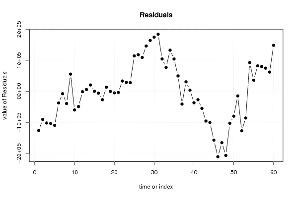
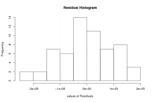
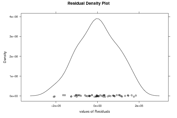
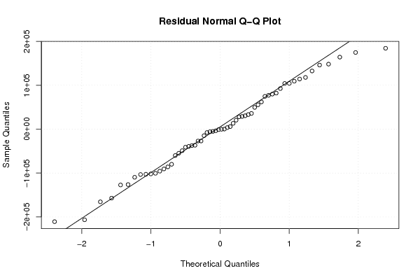
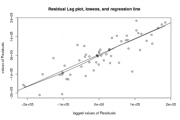
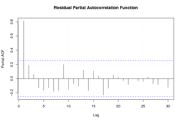
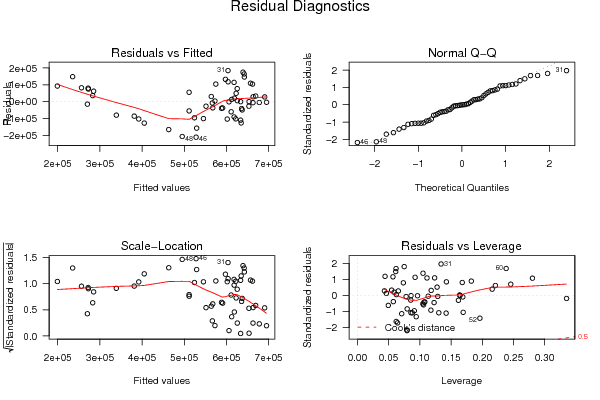
Charts produced by software:

http://www.freestatistics.org/blog/date/2010/Dec/20/t12928482855ycwglqxzond6rr/10q98z1292848335.png (open in new window) http://www.freestatistics.org/blog/date/2010/Dec/20/t12928482855ycwglqxzond6rr/10q98z1292848335.ps (open in new window) http://www.freestatistics.org/blog/date/2010/Dec/20/t12928482855ycwglqxzond6rr/1j9b61292848335.png (open in new window) http://www.freestatistics.org/blog/date/2010/Dec/20/t12928482855ycwglqxzond6rr/1j9b61292848335.ps (open in new window) http://www.freestatistics.org/blog/date/2010/Dec/20/t12928482855ycwglqxzond6rr/2c0a91292848335.png (open in new window) http://www.freestatistics.org/blog/date/2010/Dec/20/t12928482855ycwglqxzond6rr/2c0a91292848335.ps (open in new window) http://www.freestatistics.org/blog/date/2010/Dec/20/t12928482855ycwglqxzond6rr/3c0a91292848335.png (open in new window) http://www.freestatistics.org/blog/date/2010/Dec/20/t12928482855ycwglqxzond6rr/3c0a91292848335.ps (open in new window) http://www.freestatistics.org/blog/date/2010/Dec/20/t12928482855ycwglqxzond6rr/4c0a91292848335.png (open in new window) http://www.freestatistics.org/blog/date/2010/Dec/20/t12928482855ycwglqxzond6rr/4c0a91292848335.ps (open in new window) http://www.freestatistics.org/blog/date/2010/Dec/20/t12928482855ycwglqxzond6rr/54rsc1292848335.png (open in new window) http://www.freestatistics.org/blog/date/2010/Dec/20/t12928482855ycwglqxzond6rr/54rsc1292848335.ps (open in new window) http://www.freestatistics.org/blog/date/2010/Dec/20/t12928482855ycwglqxzond6rr/64rsc1292848335.png (open in new window) http://www.freestatistics.org/blog/date/2010/Dec/20/t12928482855ycwglqxzond6rr/64rsc1292848335.ps (open in new window) http://www.freestatistics.org/blog/date/2010/Dec/20/t12928482855ycwglqxzond6rr/7x09x1292848335.png (open in new window) http://www.freestatistics.org/blog/date/2010/Dec/20/t12928482855ycwglqxzond6rr/7x09x1292848335.ps (open in new window) http://www.freestatistics.org/blog/date/2010/Dec/20/t12928482855ycwglqxzond6rr/8x09x1292848335.png (open in new window) http://www.freestatistics.org/blog/date/2010/Dec/20/t12928482855ycwglqxzond6rr/8x09x1292848335.ps (open in new window) http://www.freestatistics.org/blog/date/2010/Dec/20/t12928482855ycwglqxzond6rr/9q98z1292848335.png (open in new window) http://www.freestatistics.org/blog/date/2010/Dec/20/t12928482855ycwglqxzond6rr/9q98z1292848335.ps (open in new window)

Parameters (Session):

par1 = 7 ; par2 = Do not include Seasonal Dummies ; par3 = No Linear Trend ;

Parameters (R input):

par1 = 7 ; par2 = Do not include Seasonal Dummies ; par3 = No Linear Trend ;

R code (references can be found in the software module):

library(lattice) library(lmtest) n25 <- 25 #minimum number of obs. for Goldfeld-Quandt test par1 <- as.numeric(par1) x <- t(y) k <- length(x[1,]) n <- length(x[,1]) x1 <- cbind(x[,par1], x[,1:k!=par1]) mycolnames <- c(colnames(x)[par1], colnames(x)[1:k!=par1]) colnames(x1) <- mycolnames #colnames(x)[par1] x <- x1 if (par3 == 'First Differences'){ x2 <- array(0, dim=c(n-1,k), dimnames=list(1:(n-1), paste('(1-B)',colnames(x),sep=''))) for (i in 1:n-1) { for (j in 1:k) { x2[i,j] <- x[i+1,j] - x[i,j] } } x <- x2 } if (par2 == 'Include Monthly Dummies'){ x2 <- array(0, dim=c(n,11), dimnames=list(1:n, paste('M', seq(1:11), sep =''))) for (i in 1:11){ x2[seq(i,n,12),i] <- 1 } x <- cbind(x, x2) } if (par2 == 'Include Quarterly Dummies'){ x2 <- array(0, dim=c(n,3), dimnames=list(1:n, paste('Q', seq(1:3), sep =''))) for (i in 1:3){ x2[seq(i,n,4),i] <- 1 } x <- cbind(x, x2) } k <- length(x[1,]) if (par3 == 'Linear Trend'){ x <- cbind(x, c(1:n)) colnames(x)[k+1] <- 't' } x k <- length(x[1,]) df <- as.data.frame(x) (mylm <- lm(df)) (mysum <- summary(mylm)) if (n > n25) { kp3 <- k + 3 nmkm3 <- n - k - 3 gqarr <- array(NA, dim=c(nmkm3-kp3+1,3)) numgqtests <- 0 numsignificant1 <- 0 numsignificant5 <- 0 numsignificant10 <- 0 for (mypoint in kp3:nmkm3) { j <- 0 numgqtests <- numgqtests + 1 for (myalt in c('greater', 'two.sided', 'less')) { j <- j + 1 gqarr[mypoint-kp3+1,j] <- gqtest(mylm, point=mypoint, alternative=myalt)$p.value } if (gqarr[mypoint-kp3+1,2] < 0.01) numsignificant1 <- numsignificant1 + 1 if (gqarr[mypoint-kp3+1,2] < 0.05) numsignificant5 <- numsignificant5 + 1 if (gqarr[mypoint-kp3+1,2] < 0.10) numsignificant10 <- numsignificant10 + 1 } gqarr } bitmap(file='test0.png') plot(x[,1], type='l', main='Actuals and Interpolation', ylab='value of Actuals and Interpolation (dots)', xlab='time or index') points(x[,1]-mysum$resid) grid() dev.off() bitmap(file='test1.png') plot(mysum$resid, type='b', pch=19, main='Residuals', ylab='value of Residuals', xlab='time or index') grid() dev.off() bitmap(file='test2.png') hist(mysum$resid, main='Residual Histogram', xlab='values of Residuals') grid() dev.off() bitmap(file='test3.png') densityplot(~mysum$resid,col='black',main='Residual Density Plot', xlab='values of Residuals') dev.off() bitmap(file='test4.png') qqnorm(mysum$resid, main='Residual Normal Q-Q Plot') qqline(mysum$resid) grid() dev.off() (myerror <- as.ts(mysum$resid)) bitmap(file='test5.png') dum <- cbind(lag(myerror,k=1),myerror) dum dum1 <- dum[2:length(myerror),] dum1 z <- as.data.frame(dum1) z plot(z,main=paste('Residual Lag plot, lowess, and regression line'), ylab='values of Residuals', xlab='lagged values of Residuals') lines(lowess(z)) abline(lm(z)) grid() dev.off() bitmap(file='test6.png') acf(mysum$resid, lag.max=length(mysum$resid)/2, main='Residual Autocorrelation Function') grid() dev.off() bitmap(file='test7.png') pacf(mysum$resid, lag.max=length(mysum$resid)/2, main='Residual Partial Autocorrelation Function') grid() dev.off() bitmap(file='test8.png') opar <- par(mfrow = c(2,2), oma = c(0, 0, 1.1, 0)) plot(mylm, las = 1, sub='Residual Diagnostics') par(opar) dev.off() if (n > n25) { bitmap(file='test9.png') plot(kp3:nmkm3,gqarr[,2], main='Goldfeld-Quandt test',ylab='2-sided p-value',xlab='breakpoint') grid() dev.off() } load(file='createtable') a<-table.start() a<-table.row.start(a) a<-table.element(a, 'Multiple Linear Regression - Estimated Regression Equation', 1, TRUE) a<-table.row.end(a) myeq <- colnames(x)[1] myeq <- paste(myeq, '[t] = ', sep='') for (i in 1:k){ if (mysum$coefficients[i,1] > 0) myeq <- paste(myeq, '+', '') myeq <- paste(myeq, mysum$coefficients[i,1], sep=' ') if (rownames(mysum$coefficients)[i] != '(Intercept)') { myeq <- paste(myeq, rownames(mysum$coefficients)[i], sep='') if (rownames(mysum$coefficients)[i] != 't') myeq <- paste(myeq, '[t]', sep='') } } myeq <- paste(myeq, ' + e[t]') a<-table.row.start(a) a<-table.element(a, myeq) a<-table.row.end(a) a<-table.end(a) table.save(a,file='mytable1.tab') a<-table.start() a<-table.row.start(a) a<-table.element(a,hyperlink('http://www.xycoon.com/ols1.htm','Multiple Linear Regression - Ordinary Least Squares',''), 6, TRUE) a<-table.row.end(a) a<-table.row.start(a) a<-table.element(a,'Variable',header=TRUE) a<-table.element(a,'Parameter',header=TRUE) a<-table.element(a,'S.D.',header=TRUE) a<-table.element(a,'T-STAT<br />H0: parameter = 0',header=TRUE) a<-table.element(a,'2-tail p-value',header=TRUE) a<-table.element(a,'1-tail p-value',header=TRUE) a<-table.row.end(a) for (i in 1:k){ a<-table.row.start(a) a<-table.element(a,rownames(mysum$coefficients)[i],header=TRUE) a<-table.element(a,mysum$coefficients[i,1]) a<-table.element(a, round(mysum$coefficients[i,2],6)) a<-table.element(a, round(mysum$coefficients[i,3],4)) a<-table.element(a, round(mysum$coefficients[i,4],6)) a<-table.element(a, round(mysum$coefficients[i,4]/2,6)) a<-table.row.end(a) } a<-table.end(a) table.save(a,file='mytable2.tab') a<-table.start() a<-table.row.start(a) a<-table.element(a, 'Multiple Linear Regression - Regression Statistics', 2, TRUE) a<-table.row.end(a) a<-table.row.start(a) a<-table.element(a, 'Multiple R',1,TRUE) a<-table.element(a, sqrt(mysum$r.squared)) a<-table.row.end(a) a<-table.row.start(a) a<-table.element(a, 'R-squared',1,TRUE) a<-table.element(a, mysum$r.squared) a<-table.row.end(a) a<-table.row.start(a) a<-table.element(a, 'Adjusted R-squared',1,TRUE) a<-table.element(a, mysum$adj.r.squared) a<-table.row.end(a) a<-table.row.start(a) a<-table.element(a, 'F-TEST (value)',1,TRUE) a<-table.element(a, mysum$fstatistic[1]) a<-table.row.end(a) a<-table.row.start(a) a<-table.element(a, 'F-TEST (DF numerator)',1,TRUE) a<-table.element(a, mysum$fstatistic[2]) a<-table.row.end(a) a<-table.row.start(a) a<-table.element(a, 'F-TEST (DF denominator)',1,TRUE) a<-table.element(a, mysum$fstatistic[3]) a<-table.row.end(a) a<-table.row.start(a) a<-table.element(a, 'p-value',1,TRUE) a<-table.element(a, 1-pf(mysum$fstatistic[1],mysum$fstatistic[2],mysum$fstatistic[3])) a<-table.row.end(a) a<-table.row.start(a) a<-table.element(a, 'Multiple Linear Regression - Residual Statistics', 2, TRUE) a<-table.row.end(a) a<-table.row.start(a) a<-table.element(a, 'Residual Standard Deviation',1,TRUE) a<-table.element(a, mysum$sigma) a<-table.row.end(a) a<-table.row.start(a) a<-table.element(a, 'Sum Squared Residuals',1,TRUE) a<-table.element(a, sum(myerror*myerror)) a<-table.row.end(a) a<-table.end(a) table.save(a,file='mytable3.tab') a<-table.start() a<-table.row.start(a) a<-table.element(a, 'Multiple Linear Regression - Actuals, Interpolation, and Residuals', 4, TRUE) a<-table.row.end(a) a<-table.row.start(a) a<-table.element(a, 'Time or Index', 1, TRUE) a<-table.element(a, 'Actuals', 1, TRUE) a<-table.element(a, 'Interpolation<br />Forecast', 1, TRUE) a<-table.element(a, 'Residuals<br />Prediction Error', 1, TRUE) a<-table.row.end(a) for (i in 1:n) { a<-table.row.start(a) a<-table.element(a,i, 1, TRUE) a<-table.element(a,x[i]) a<-table.element(a,x[i]-mysum$resid[i]) a<-table.element(a,mysum$resid[i]) a<-table.row.end(a) } a<-table.end(a) table.save(a,file='mytable4.tab') if (n > n25) { a<-table.start() a<-table.row.start(a) a<-table.element(a,'Goldfeld-Quandt test for Heteroskedasticity',4,TRUE) a<-table.row.end(a) a<-table.row.start(a) a<-table.element(a,'p-values',header=TRUE) a<-table.element(a,'Alternative Hypothesis',3,header=TRUE) a<-table.row.end(a) a<-table.row.start(a) a<-table.element(a,'breakpoint index',header=TRUE) a<-table.element(a,'greater',header=TRUE) a<-table.element(a,'2-sided',header=TRUE) a<-table.element(a,'less',header=TRUE) a<-table.row.end(a) for (mypoint in kp3:nmkm3) { a<-table.row.start(a) a<-table.element(a,mypoint,header=TRUE) a<-table.element(a,gqarr[mypoint-kp3+1,1]) a<-table.element(a,gqarr[mypoint-kp3+1,2]) a<-table.element(a,gqarr[mypoint-kp3+1,3]) a<-table.row.end(a) } a<-table.end(a) table.save(a,file='mytable5.tab') a<-table.start() a<-table.row.start(a) a<-table.element(a,'Meta Analysis of Goldfeld-Quandt test for Heteroskedasticity',4,TRUE) a<-table.row.end(a) a<-table.row.start(a) a<-table.element(a,'Description',header=TRUE) a<-table.element(a,'# significant tests',header=TRUE) a<-table.element(a,'% significant tests',header=TRUE) a<-table.element(a,'OK/NOK',header=TRUE) a<-table.row.end(a) a<-table.row.start(a) a<-table.element(a,'1% type I error level',header=TRUE) a<-table.element(a,numsignificant1) a<-table.element(a,numsignificant1/numgqtests) if (numsignificant1/numgqtests < 0.01) dum <- 'OK' else dum <- 'NOK' a<-table.element(a,dum) a<-table.row.end(a) a<-table.row.start(a) a<-table.element(a,'5% type I error level',header=TRUE) a<-table.element(a,numsignificant5) a<-table.element(a,numsignificant5/numgqtests) if (numsignificant5/numgqtests < 0.05) dum <- 'OK' else dum <- 'NOK' a<-table.element(a,dum) a<-table.row.end(a) a<-table.row.start(a) a<-table.element(a,'10% type I error level',header=TRUE) a<-table.element(a,numsignificant10) a<-table.element(a,numsignificant10/numgqtests) if (numsignificant10/numgqtests < 0.1) dum <- 'OK' else dum <- 'NOK' a<-table.element(a,dum) a<-table.row.end(a) a<-table.end(a) table.save(a,file='mytable6.tab') }

Copyright

This work is licensed under a Creative Commons Attribution-Noncommercial-Share Alike 3.0 License.

Software written by Ed van Stee & Patrick Wessa

Disclaimer

Information provided on this web site is provided "AS IS" without warranty of any kind, either express or implied, including, without limitation, warranties of merchantability, fitness for a particular purpose, and noninfringement. We use reasonable efforts to include accurate and timely information and periodically update the information, and software without notice. However, we make no warranties or representations as to the accuracy or completeness of such information (or software), and we assume no liability or responsibility for errors or omissions in the content of this web site, or any software bugs in online applications. Your use of this web site is AT YOUR OWN RISK. Under no circumstances and under no legal theory shall we be liable to you or any other person for any direct, indirect, special, incidental, exemplary, or consequential damages arising from your access to, or use of, this web site.

Privacy Policy

We may request personal information to be submitted to our servers in order to be able to:

• personalize online software applications according to your needs
• enforce strict security rules with respect to the data that you upload (e.g. statistical data)
• manage user sessions of online applications
• alert you about important changes or upgrades in resources or applications

We NEVER allow other companies to directly offer registered users information about their products and services. Banner references and hyperlinks of third parties NEVER contain any personal data of the visitor.

We do NOT sell, nor transmit by any means, personal information, nor statistical data series uploaded by you to third parties.

We carefully protect your data from loss, misuse, alteration, and destruction. However, at any time, and under any circumstance you are solely responsible for managing your passwords, and keeping them secret.

We store a unique ANONYMOUS USER ID in the form of a small 'Cookie' on your computer. This allows us to track your progress when using this website which is necessary to create state-dependent features. The cookie is used for NO OTHER PURPOSE. At any time you may opt to disallow cookies from this website - this will not affect other features of this website.

We examine cookies that are used by third-parties (banner and online ads) very closely: abuse from third-parties automatically results in termination of the advertising contract without refund. We have very good reason to believe that the cookies that are produced by third parties (banner ads) do NOT cause any privacy or security risk.

FreeStatistics.org is safe. There is no need to download any software to use the applications and services contained in this website. Hence, your system's security is not compromised by their use, and your personal data - other than data you submit in the account application form, and the user-agent information that is transmitted by your browser - is never transmitted to our servers.

As a general rule, we do not log on-line behavior of individuals (other than normal logging of webserver 'hits'). However, in cases of abuse, hacking, unauthorized access, Denial of Service attacks, illegal copying, hotlinking, non-compliance with international webstandards (such as robots.txt), or any other harmful behavior, our system engineers are empowered to log, track, identify, publish, and ban misbehaving individuals - even if this leads to ban entire blocks of IP addresses, or disclosing user's identity.

FreeStatistics.org is powered by