Free Statistics
of Irreproducible Research!
Description of Statistical Computation | |||||||||||||||||||||||||||||||||||||||||||||||||||||||||||||
|---|---|---|---|---|---|---|---|---|---|---|---|---|---|---|---|---|---|---|---|---|---|---|---|---|---|---|---|---|---|---|---|---|---|---|---|---|---|---|---|---|---|---|---|---|---|---|---|---|---|---|---|---|---|---|---|---|---|---|---|---|---|
| Author's title | |||||||||||||||||||||||||||||||||||||||||||||||||||||||||||||
| Author | *The author of this computation has been verified* | ||||||||||||||||||||||||||||||||||||||||||||||||||||||||||||
| R Software Module | rwasp_linear_regression.wasp | ||||||||||||||||||||||||||||||||||||||||||||||||||||||||||||
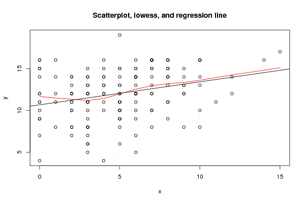
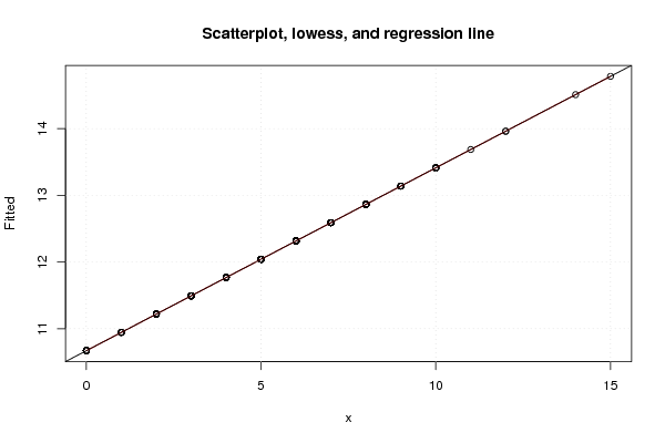
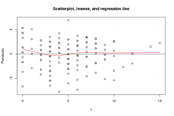
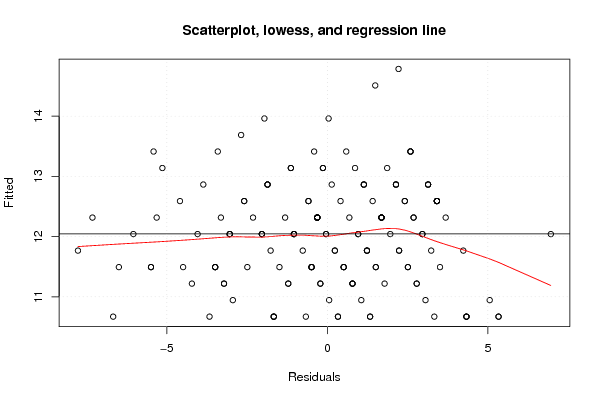
| Title produced by software | Linear Regression Graphical Model Validation | ||||||||||||||||||||||||||||||||||||||||||||||||||||||||||||
| Date of computation | Mon, 20 Dec 2010 10:23:31 +0000 | ||||||||||||||||||||||||||||||||||||||||||||||||||||||||||||
| Cite this page as follows | Statistical Computations at FreeStatistics.org, Office for Research Development and Education, URL https://freestatistics.org/blog/index.php?v=date/2010/Dec/20/t1292840743po6kwh0gu9md424.htm/, Retrieved Thu, 18 Sep 2025 01:50:37 +0000 | ||||||||||||||||||||||||||||||||||||||||||||||||||||||||||||
| Statistical Computations at FreeStatistics.org, Office for Research Development and Education, URL https://freestatistics.org/blog/index.php?pk=112831, Retrieved Thu, 18 Sep 2025 01:50:37 +0000 | |||||||||||||||||||||||||||||||||||||||||||||||||||||||||||||
| QR Codes: | |||||||||||||||||||||||||||||||||||||||||||||||||||||||||||||
|
| |||||||||||||||||||||||||||||||||||||||||||||||||||||||||||||
| Original text written by user: | |||||||||||||||||||||||||||||||||||||||||||||||||||||||||||||
| IsPrivate? | No (this computation is public) | ||||||||||||||||||||||||||||||||||||||||||||||||||||||||||||
| User-defined keywords | |||||||||||||||||||||||||||||||||||||||||||||||||||||||||||||
| Estimated Impact | 311 | ||||||||||||||||||||||||||||||||||||||||||||||||||||||||||||
Tree of Dependent Computations | |||||||||||||||||||||||||||||||||||||||||||||||||||||||||||||
| Family? (F = Feedback message, R = changed R code, M = changed R Module, P = changed Parameters, D = changed Data) | |||||||||||||||||||||||||||||||||||||||||||||||||||||||||||||
| - [Linear Regression Graphical Model Validation] [Mini tutorial] [2010-11-11 13:04:30] [1fd136673b2a4fecb5c545b9b4a05d64] - D [Linear Regression Graphical Model Validation] [ws6.mini hypothese 1] [2010-11-15 18:16:27] [e4076051fbfb461c886b1e223cd7862f] - D [Linear Regression Graphical Model Validation] [PAPER BAEYENS (Li...] [2010-12-20 10:12:09] [e4076051fbfb461c886b1e223cd7862f] - D [Linear Regression Graphical Model Validation] [PAPER BAEYENS (Li...] [2010-12-20 10:23:31] [2953e4eb3235e2fd3d6373a16d27c72f] [Current] | |||||||||||||||||||||||||||||||||||||||||||||||||||||||||||||
| Feedback Forum | |||||||||||||||||||||||||||||||||||||||||||||||||||||||||||||
Post a new message | |||||||||||||||||||||||||||||||||||||||||||||||||||||||||||||
Dataset | |||||||||||||||||||||||||||||||||||||||||||||||||||||||||||||
| Dataseries X: | |||||||||||||||||||||||||||||||||||||||||||||||||||||||||||||
5 3 0 7 4 1 6 3 12 0 5 6 6 6 2 1 5 7 3 3 3 7 8 6 3 5 5 10 2 6 4 6 8 4 5 10 6 7 4 10 4 3 3 3 3 7 15 0 0 4 5 5 2 3 0 9 2 7 7 0 0 10 2 1 8 6 11 3 8 6 9 9 8 8 7 6 5 4 6 3 2 12 8 5 9 6 5 2 4 7 5 6 7 8 6 0 1 5 5 5 7 7 1 3 4 8 6 6 2 2 3 3 0 2 8 8 0 5 9 6 6 3 9 7 8 0 7 0 5 0 14 5 2 8 4 2 6 3 5 9 3 3 0 10 4 2 3 10 7 0 6 8 0 4 10 5 | |||||||||||||||||||||||||||||||||||||||||||||||||||||||||||||
| Dataseries Y: | |||||||||||||||||||||||||||||||||||||||||||||||||||||||||||||
13 12 15 12 10 12 15 9 12 11 11 11 15 7 11 11 10 14 10 6 11 15 11 12 14 15 9 13 13 16 13 12 14 11 9 16 12 10 13 16 14 15 5 8 11 16 17 9 9 13 10 6 12 8 14 12 11 16 8 15 7 16 14 16 9 14 11 13 15 5 15 13 11 11 12 12 12 12 14 6 7 14 14 10 13 12 9 12 16 10 14 10 16 15 12 10 8 8 11 13 16 16 14 11 4 14 9 14 8 8 11 12 11 14 15 16 16 11 14 14 12 14 8 13 16 12 16 12 11 4 16 15 10 13 15 12 14 7 19 12 12 13 15 8 12 10 8 10 15 16 13 16 9 14 14 12 | |||||||||||||||||||||||||||||||||||||||||||||||||||||||||||||
Tables (Output of Computation) | |||||||||||||||||||||||||||||||||||||||||||||||||||||||||||||
| |||||||||||||||||||||||||||||||||||||||||||||||||||||||||||||
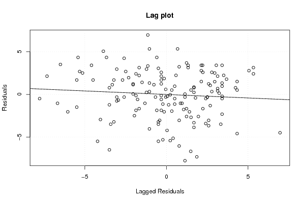
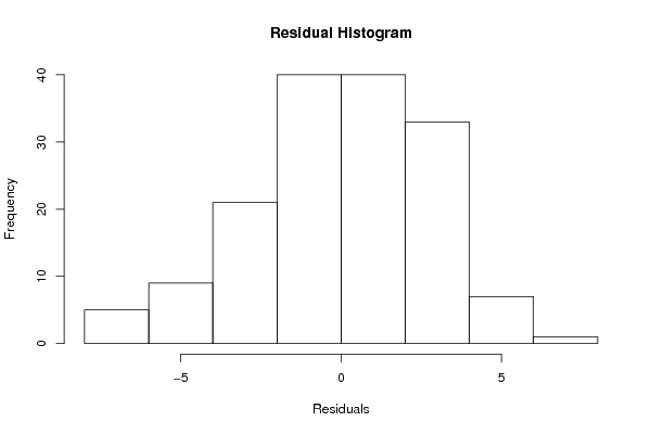
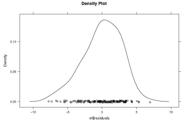
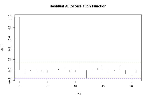
Figures (Output of Computation) | |||||||||||||||||||||||||||||||||||||||||||||||||||||||||||||
Input Parameters & R Code | |||||||||||||||||||||||||||||||||||||||||||||||||||||||||||||
| Parameters (Session): | |||||||||||||||||||||||||||||||||||||||||||||||||||||||||||||
| par1 = 0 ; | |||||||||||||||||||||||||||||||||||||||||||||||||||||||||||||
| Parameters (R input): | |||||||||||||||||||||||||||||||||||||||||||||||||||||||||||||
| par1 = 0 ; | |||||||||||||||||||||||||||||||||||||||||||||||||||||||||||||
| R code (references can be found in the software module): | |||||||||||||||||||||||||||||||||||||||||||||||||||||||||||||
par1 <- as.numeric(par1) | |||||||||||||||||||||||||||||||||||||||||||||||||||||||||||||