Repository of Reproducible Computations

Free Statistics

of Irreproducible Research!

Author's title

Author

*The author of this computation has been verified*

R Software Module

rwasp_autocorrelation.wasp

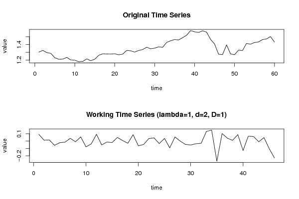
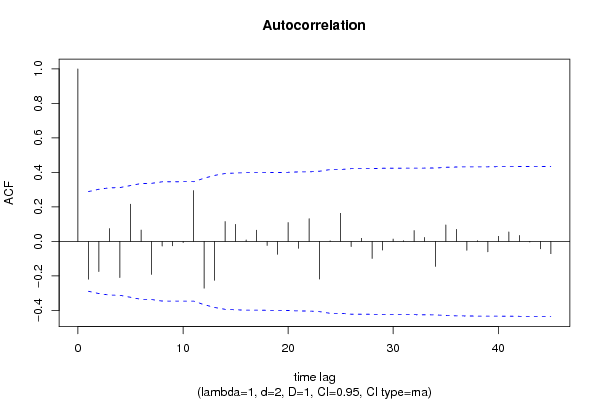
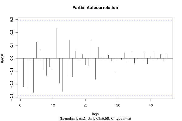
Title produced by software

(Partial) Autocorrelation Function

Date of computation

Fri, 17 Dec 2010 15:00:38 +0000

Cite this page as follows

Statistical Computations at FreeStatistics.org, Office for Research Development and Education, URL https://freestatistics.org/blog/index.php?v=date/2010/Dec/17/t12925980701zzvww5ek1rfwdo.htm/, Retrieved Wed, 01 May 2024 22:45:12 +0000

Statistical Computations at FreeStatistics.org, Office for Research Development and Education, URL https://freestatistics.org/blog/index.php?pk=111509, Retrieved Wed, 01 May 2024 22:45:12 +0000

QR Codes:

Paste this QR Code to cite your computation.

Original text written by user:

IsPrivate?

No (this computation is public)

User-defined keywords

Estimated Impact

136

Family? (F = Feedback message, R = changed R code, M = changed R Module, P = changed Parameters, D = changed Data)

-     [Univariate Explorative Data Analysis] [Run Sequence gebo...] [2008-12-12 13:32:37] [76963dc1903f0f612b6153510a3818cf]
- R  D  [Univariate Explorative Data Analysis] [Run Sequence gebo...] [2008-12-17 12:14:40] [76963dc1903f0f612b6153510a3818cf]
-         [Univariate Explorative Data Analysis] [Run Sequence Plot...] [2008-12-22 18:19:51] [1ce0d16c8f4225c977b42c8fa93bc163]
- RMP       [(Partial) Autocorrelation Function] [Identifying Integ...] [2009-11-22 12:16:10] [b98453cac15ba1066b407e146608df68]
-    D        [(Partial) Autocorrelation Function] [Model 1 (d = 0, D...] [2009-11-24 17:27:24] [ee7c2e7343f5b1451e62c5c16ec521f1]
-    D          [(Partial) Autocorrelation Function] [Methode 1 (D=0, d=0)] [2009-11-27 12:01:23] [76ab39dc7a55316678260825bd5ad46c]
-    D            [(Partial) Autocorrelation Function] [methode 1 (d=0 D= 0)] [2009-11-27 20:21:42] [4b453aa14d54730625f8d3de5f1f6d82]
-    D              [(Partial) Autocorrelation Function] [koffie en thee] [2009-12-16 19:04:55] [7773f496f69461f4a67891f0ef752622]
-    D                [(Partial) Autocorrelation Function] [Appelen Jonagold ...] [2009-12-17 16:51:16] [7773f496f69461f4a67891f0ef752622]
- R PD                  [(Partial) Autocorrelation Function] [autocorrelatie] [2010-12-15 16:41:13] [717f3d787904f94c39256c5c1fc72d4c]
-   P                       [(Partial) Autocorrelation Function] [autocorrelatie d=...] [2010-12-17 15:00:38] [c1f1b5e209adb4577289f490325e36f2] [Current]

Feedback Forum

Post a new message

Dataseries X:

Download CSV

Histogram

Boxplots

Summary of computational transaction
Raw Input	view raw input (R code)
Raw Output	view raw output of R engine
Computing time	2 seconds
R Server	'Gwilym Jenkins' @ 72.249.127.135

\begin{tabular}{lllllllll}
\hline
Summary of computational transaction \tabularnewline
Raw Input & view raw input (R code)  \tabularnewline
Raw Output & view raw output of R engine  \tabularnewline
Computing time & 2 seconds \tabularnewline
R Server & 'Gwilym Jenkins' @ 72.249.127.135 \tabularnewline
\hline
\end{tabular}
%Source: https://freestatistics.org/blog/index.php?pk=111509&T=0

[TABLE]
[ROW][C]Summary of computational transaction[/C][/ROW]
[ROW][C]Raw Input[/C][C]view raw input (R code) [/C][/ROW]
[ROW][C]Raw Output[/C][C]view raw output of R engine [/C][/ROW]
[ROW][C]Computing time[/C][C]2 seconds[/C][/ROW]
[ROW][C]R Server[/C][C]'Gwilym Jenkins' @ 72.249.127.135[/C][/ROW]
[/TABLE]
Source: https://freestatistics.org/blog/index.php?pk=111509&T=0

Globally Unique Identifier (entire table): ba.freestatistics.org/blog/index.php?pk=111509&T=0

As an alternative you can also use a QR Code:

The GUIDs for individual cells are displayed in the table below:

Summary of computational transaction
Raw Input	view raw input (R code)
Raw Output	view raw output of R engine
Computing time	2 seconds
R Server	'Gwilym Jenkins' @ 72.249.127.135

Autocorrelation Function
Time lag k	ACF(k)	T-STAT	P-value
1	-0.219112	-1.4861	0.072039
2	-0.174439	-1.1831	0.121424
3	0.074636	0.5062	0.307566
4	-0.209886	-1.4235	0.080668
5	0.215908	1.4644	0.074949
6	0.065912	0.447	0.328473
7	-0.19172	-1.3003	0.099987
8	-0.02674	-0.1814	0.428442
9	-0.025262	-0.1713	0.432356
10	-0.006795	-0.0461	0.481721
11	0.295132	2.0017	0.025619
12	-0.270992	-1.838	0.036266
13	-0.225425	-1.5289	0.066568
14	0.115431	0.7829	0.218852
15	0.098853	0.6705	0.252961
16	0.008441	0.0573	0.477296
17	0.06529	0.4428	0.329987
18	-0.023312	-0.1581	0.43753
19	-0.074833	-0.5075	0.307099
20	0.109368	0.7418	0.230999
21	-0.040155	-0.2723	0.393288
22	0.131989	0.8952	0.187673
23	-0.218418	-1.4814	0.072662
24	0.003644	0.0247	0.490195
25	0.16324	1.1072	0.136993
26	-0.029938	-0.2031	0.419995
27	0.018018	0.1222	0.451635
28	-0.098464	-0.6678	0.253795
29	-0.050296	-0.3411	0.367282
30	0.013751	0.0933	0.463049
31	0.004329	0.0294	0.488352
32	0.063195	0.4286	0.335103
33	0.023348	0.1584	0.437437
34	-0.145352	-0.9858	0.164688
35	0.095466	0.6475	0.26027
36	0.069868	0.4739	0.318919
37	-0.051621	-0.3501	0.363926
38	0.004277	0.029	0.488491
39	-0.060236	-0.4085	0.342387
40	0.029969	0.2033	0.419915
41	0.055059	0.3734	0.355272
42	0.035015	0.2375	0.406669
43	-0.003556	-0.0241	0.490431
44	-0.042757	-0.29	0.386562
45	-0.070828	-0.4804	0.316618
46	NA	NA	NA
47	NA	NA	NA
48	NA	NA	NA
49	NA	NA	NA
50	NA	NA	NA
51	NA	NA	NA
52	NA	NA	NA
53	NA	NA	NA
54	NA	NA	NA
55	NA	NA	NA
56	NA	NA	NA
57	NA	NA	NA
58	NA	NA	NA
59	NA	NA	NA
60	NA	NA	NA

\begin{tabular}{lllllllll}
\hline
Autocorrelation Function \tabularnewline
Time lag k & ACF(k) & T-STAT & P-value \tabularnewline
1 & -0.219112 & -1.4861 & 0.072039 \tabularnewline
2 & -0.174439 & -1.1831 & 0.121424 \tabularnewline
3 & 0.074636 & 0.5062 & 0.307566 \tabularnewline
4 & -0.209886 & -1.4235 & 0.080668 \tabularnewline
5 & 0.215908 & 1.4644 & 0.074949 \tabularnewline
6 & 0.065912 & 0.447 & 0.328473 \tabularnewline
7 & -0.19172 & -1.3003 & 0.099987 \tabularnewline
8 & -0.02674 & -0.1814 & 0.428442 \tabularnewline
9 & -0.025262 & -0.1713 & 0.432356 \tabularnewline
10 & -0.006795 & -0.0461 & 0.481721 \tabularnewline
11 & 0.295132 & 2.0017 & 0.025619 \tabularnewline
12 & -0.270992 & -1.838 & 0.036266 \tabularnewline
13 & -0.225425 & -1.5289 & 0.066568 \tabularnewline
14 & 0.115431 & 0.7829 & 0.218852 \tabularnewline
15 & 0.098853 & 0.6705 & 0.252961 \tabularnewline
16 & 0.008441 & 0.0573 & 0.477296 \tabularnewline
17 & 0.06529 & 0.4428 & 0.329987 \tabularnewline
18 & -0.023312 & -0.1581 & 0.43753 \tabularnewline
19 & -0.074833 & -0.5075 & 0.307099 \tabularnewline
20 & 0.109368 & 0.7418 & 0.230999 \tabularnewline
21 & -0.040155 & -0.2723 & 0.393288 \tabularnewline
22 & 0.131989 & 0.8952 & 0.187673 \tabularnewline
23 & -0.218418 & -1.4814 & 0.072662 \tabularnewline
24 & 0.003644 & 0.0247 & 0.490195 \tabularnewline
25 & 0.16324 & 1.1072 & 0.136993 \tabularnewline
26 & -0.029938 & -0.2031 & 0.419995 \tabularnewline
27 & 0.018018 & 0.1222 & 0.451635 \tabularnewline
28 & -0.098464 & -0.6678 & 0.253795 \tabularnewline
29 & -0.050296 & -0.3411 & 0.367282 \tabularnewline
30 & 0.013751 & 0.0933 & 0.463049 \tabularnewline
31 & 0.004329 & 0.0294 & 0.488352 \tabularnewline
32 & 0.063195 & 0.4286 & 0.335103 \tabularnewline
33 & 0.023348 & 0.1584 & 0.437437 \tabularnewline
34 & -0.145352 & -0.9858 & 0.164688 \tabularnewline
35 & 0.095466 & 0.6475 & 0.26027 \tabularnewline
36 & 0.069868 & 0.4739 & 0.318919 \tabularnewline
37 & -0.051621 & -0.3501 & 0.363926 \tabularnewline
38 & 0.004277 & 0.029 & 0.488491 \tabularnewline
39 & -0.060236 & -0.4085 & 0.342387 \tabularnewline
40 & 0.029969 & 0.2033 & 0.419915 \tabularnewline
41 & 0.055059 & 0.3734 & 0.355272 \tabularnewline
42 & 0.035015 & 0.2375 & 0.406669 \tabularnewline
43 & -0.003556 & -0.0241 & 0.490431 \tabularnewline
44 & -0.042757 & -0.29 & 0.386562 \tabularnewline
45 & -0.070828 & -0.4804 & 0.316618 \tabularnewline
46 & NA & NA & NA \tabularnewline
47 & NA & NA & NA \tabularnewline
48 & NA & NA & NA \tabularnewline
49 & NA & NA & NA \tabularnewline
50 & NA & NA & NA \tabularnewline
51 & NA & NA & NA \tabularnewline
52 & NA & NA & NA \tabularnewline
53 & NA & NA & NA \tabularnewline
54 & NA & NA & NA \tabularnewline
55 & NA & NA & NA \tabularnewline
56 & NA & NA & NA \tabularnewline
57 & NA & NA & NA \tabularnewline
58 & NA & NA & NA \tabularnewline
59 & NA & NA & NA \tabularnewline
60 & NA & NA & NA \tabularnewline
\hline
\end{tabular}
%Source: https://freestatistics.org/blog/index.php?pk=111509&T=1

[TABLE]
[ROW][C]Autocorrelation Function[/C][/ROW]
[ROW][C]Time lag k[/C][C]ACF(k)[/C][C]T-STAT[/C][C]P-value[/C][/ROW]
[ROW][C]1[/C][C]-0.219112[/C][C]-1.4861[/C][C]0.072039[/C][/ROW]
[ROW][C]2[/C][C]-0.174439[/C][C]-1.1831[/C][C]0.121424[/C][/ROW]
[ROW][C]3[/C][C]0.074636[/C][C]0.5062[/C][C]0.307566[/C][/ROW]
[ROW][C]4[/C][C]-0.209886[/C][C]-1.4235[/C][C]0.080668[/C][/ROW]
[ROW][C]5[/C][C]0.215908[/C][C]1.4644[/C][C]0.074949[/C][/ROW]
[ROW][C]6[/C][C]0.065912[/C][C]0.447[/C][C]0.328473[/C][/ROW]
[ROW][C]7[/C][C]-0.19172[/C][C]-1.3003[/C][C]0.099987[/C][/ROW]
[ROW][C]8[/C][C]-0.02674[/C][C]-0.1814[/C][C]0.428442[/C][/ROW]
[ROW][C]9[/C][C]-0.025262[/C][C]-0.1713[/C][C]0.432356[/C][/ROW]
[ROW][C]10[/C][C]-0.006795[/C][C]-0.0461[/C][C]0.481721[/C][/ROW]
[ROW][C]11[/C][C]0.295132[/C][C]2.0017[/C][C]0.025619[/C][/ROW]
[ROW][C]12[/C][C]-0.270992[/C][C]-1.838[/C][C]0.036266[/C][/ROW]
[ROW][C]13[/C][C]-0.225425[/C][C]-1.5289[/C][C]0.066568[/C][/ROW]
[ROW][C]14[/C][C]0.115431[/C][C]0.7829[/C][C]0.218852[/C][/ROW]
[ROW][C]15[/C][C]0.098853[/C][C]0.6705[/C][C]0.252961[/C][/ROW]
[ROW][C]16[/C][C]0.008441[/C][C]0.0573[/C][C]0.477296[/C][/ROW]
[ROW][C]17[/C][C]0.06529[/C][C]0.4428[/C][C]0.329987[/C][/ROW]
[ROW][C]18[/C][C]-0.023312[/C][C]-0.1581[/C][C]0.43753[/C][/ROW]
[ROW][C]19[/C][C]-0.074833[/C][C]-0.5075[/C][C]0.307099[/C][/ROW]
[ROW][C]20[/C][C]0.109368[/C][C]0.7418[/C][C]0.230999[/C][/ROW]
[ROW][C]21[/C][C]-0.040155[/C][C]-0.2723[/C][C]0.393288[/C][/ROW]
[ROW][C]22[/C][C]0.131989[/C][C]0.8952[/C][C]0.187673[/C][/ROW]
[ROW][C]23[/C][C]-0.218418[/C][C]-1.4814[/C][C]0.072662[/C][/ROW]
[ROW][C]24[/C][C]0.003644[/C][C]0.0247[/C][C]0.490195[/C][/ROW]
[ROW][C]25[/C][C]0.16324[/C][C]1.1072[/C][C]0.136993[/C][/ROW]
[ROW][C]26[/C][C]-0.029938[/C][C]-0.2031[/C][C]0.419995[/C][/ROW]
[ROW][C]27[/C][C]0.018018[/C][C]0.1222[/C][C]0.451635[/C][/ROW]
[ROW][C]28[/C][C]-0.098464[/C][C]-0.6678[/C][C]0.253795[/C][/ROW]
[ROW][C]29[/C][C]-0.050296[/C][C]-0.3411[/C][C]0.367282[/C][/ROW]
[ROW][C]30[/C][C]0.013751[/C][C]0.0933[/C][C]0.463049[/C][/ROW]
[ROW][C]31[/C][C]0.004329[/C][C]0.0294[/C][C]0.488352[/C][/ROW]
[ROW][C]32[/C][C]0.063195[/C][C]0.4286[/C][C]0.335103[/C][/ROW]
[ROW][C]33[/C][C]0.023348[/C][C]0.1584[/C][C]0.437437[/C][/ROW]
[ROW][C]34[/C][C]-0.145352[/C][C]-0.9858[/C][C]0.164688[/C][/ROW]
[ROW][C]35[/C][C]0.095466[/C][C]0.6475[/C][C]0.26027[/C][/ROW]
[ROW][C]36[/C][C]0.069868[/C][C]0.4739[/C][C]0.318919[/C][/ROW]
[ROW][C]37[/C][C]-0.051621[/C][C]-0.3501[/C][C]0.363926[/C][/ROW]
[ROW][C]38[/C][C]0.004277[/C][C]0.029[/C][C]0.488491[/C][/ROW]
[ROW][C]39[/C][C]-0.060236[/C][C]-0.4085[/C][C]0.342387[/C][/ROW]
[ROW][C]40[/C][C]0.029969[/C][C]0.2033[/C][C]0.419915[/C][/ROW]
[ROW][C]41[/C][C]0.055059[/C][C]0.3734[/C][C]0.355272[/C][/ROW]
[ROW][C]42[/C][C]0.035015[/C][C]0.2375[/C][C]0.406669[/C][/ROW]
[ROW][C]43[/C][C]-0.003556[/C][C]-0.0241[/C][C]0.490431[/C][/ROW]
[ROW][C]44[/C][C]-0.042757[/C][C]-0.29[/C][C]0.386562[/C][/ROW]
[ROW][C]45[/C][C]-0.070828[/C][C]-0.4804[/C][C]0.316618[/C][/ROW]
[ROW][C]46[/C][C]NA[/C][C]NA[/C][C]NA[/C][/ROW]
[ROW][C]47[/C][C]NA[/C][C]NA[/C][C]NA[/C][/ROW]
[ROW][C]48[/C][C]NA[/C][C]NA[/C][C]NA[/C][/ROW]
[ROW][C]49[/C][C]NA[/C][C]NA[/C][C]NA[/C][/ROW]
[ROW][C]50[/C][C]NA[/C][C]NA[/C][C]NA[/C][/ROW]
[ROW][C]51[/C][C]NA[/C][C]NA[/C][C]NA[/C][/ROW]
[ROW][C]52[/C][C]NA[/C][C]NA[/C][C]NA[/C][/ROW]
[ROW][C]53[/C][C]NA[/C][C]NA[/C][C]NA[/C][/ROW]
[ROW][C]54[/C][C]NA[/C][C]NA[/C][C]NA[/C][/ROW]
[ROW][C]55[/C][C]NA[/C][C]NA[/C][C]NA[/C][/ROW]
[ROW][C]56[/C][C]NA[/C][C]NA[/C][C]NA[/C][/ROW]
[ROW][C]57[/C][C]NA[/C][C]NA[/C][C]NA[/C][/ROW]
[ROW][C]58[/C][C]NA[/C][C]NA[/C][C]NA[/C][/ROW]
[ROW][C]59[/C][C]NA[/C][C]NA[/C][C]NA[/C][/ROW]
[ROW][C]60[/C][C]NA[/C][C]NA[/C][C]NA[/C][/ROW]
[/TABLE]
Source: https://freestatistics.org/blog/index.php?pk=111509&T=1

Globally Unique Identifier (entire table): ba.freestatistics.org/blog/index.php?pk=111509&T=1

As an alternative you can also use a QR Code:

The GUIDs for individual cells are displayed in the table below:

Autocorrelation Function
Time lag k	ACF(k)	T-STAT	P-value
1	-0.219112	-1.4861	0.072039
2	-0.174439	-1.1831	0.121424
3	0.074636	0.5062	0.307566
4	-0.209886	-1.4235	0.080668
5	0.215908	1.4644	0.074949
6	0.065912	0.447	0.328473
7	-0.19172	-1.3003	0.099987
8	-0.02674	-0.1814	0.428442
9	-0.025262	-0.1713	0.432356
10	-0.006795	-0.0461	0.481721
11	0.295132	2.0017	0.025619
12	-0.270992	-1.838	0.036266
13	-0.225425	-1.5289	0.066568
14	0.115431	0.7829	0.218852
15	0.098853	0.6705	0.252961
16	0.008441	0.0573	0.477296
17	0.06529	0.4428	0.329987
18	-0.023312	-0.1581	0.43753
19	-0.074833	-0.5075	0.307099
20	0.109368	0.7418	0.230999
21	-0.040155	-0.2723	0.393288
22	0.131989	0.8952	0.187673
23	-0.218418	-1.4814	0.072662
24	0.003644	0.0247	0.490195
25	0.16324	1.1072	0.136993
26	-0.029938	-0.2031	0.419995
27	0.018018	0.1222	0.451635
28	-0.098464	-0.6678	0.253795
29	-0.050296	-0.3411	0.367282
30	0.013751	0.0933	0.463049
31	0.004329	0.0294	0.488352
32	0.063195	0.4286	0.335103
33	0.023348	0.1584	0.437437
34	-0.145352	-0.9858	0.164688
35	0.095466	0.6475	0.26027
36	0.069868	0.4739	0.318919
37	-0.051621	-0.3501	0.363926
38	0.004277	0.029	0.488491
39	-0.060236	-0.4085	0.342387
40	0.029969	0.2033	0.419915
41	0.055059	0.3734	0.355272
42	0.035015	0.2375	0.406669
43	-0.003556	-0.0241	0.490431
44	-0.042757	-0.29	0.386562
45	-0.070828	-0.4804	0.316618
46	NA	NA	NA
47	NA	NA	NA
48	NA	NA	NA
49	NA	NA	NA
50	NA	NA	NA
51	NA	NA	NA
52	NA	NA	NA
53	NA	NA	NA
54	NA	NA	NA
55	NA	NA	NA
56	NA	NA	NA
57	NA	NA	NA
58	NA	NA	NA
59	NA	NA	NA
60	NA	NA	NA

Partial Autocorrelation Function
Time lag k	PACF(k)	T-STAT	P-value
1	-0.219112	-1.4861	0.072039
2	-0.233667	-1.5848	0.059931
3	-0.026351	-0.1787	0.42947
4	-0.263544	-1.7874	0.040228
5	0.124359	0.8434	0.201672
6	0.061609	0.4179	0.338999
7	-0.089189	-0.6049	0.274105
8	-0.132442	-0.8983	0.186862
9	-0.067728	-0.4594	0.324073
10	-0.083854	-0.5687	0.286154
11	0.23406	1.5875	0.059628
12	-0.192158	-1.3033	0.099482
13	-0.255911	-1.7357	0.044659
14	-0.146477	-0.9935	0.162843
15	0.138551	0.9397	0.176141
16	-0.142861	-0.9689	0.168824
17	0.057605	0.3907	0.348912
18	0.144502	0.9801	0.166092
19	0.029563	0.2005	0.420984
20	-0.052566	-0.3565	0.36154
21	-0.059482	-0.4034	0.344252
22	0.133231	0.9036	0.185454
23	-0.162791	-1.1041	0.137646
24	0.084913	0.5759	0.283743
25	0.010138	0.0688	0.472739
26	0.00133	0.009	0.496422
27	0.025406	0.1723	0.431974
28	-0.021745	-0.1475	0.441698
29	-0.093753	-0.6359	0.264009
30	0.011982	0.0813	0.46779
31	-0.008845	-0.06	0.476211
32	0.043942	0.298	0.383512
33	-0.031195	-0.2116	0.416688
34	0.046579	0.3159	0.376748
35	-0.038083	-0.2583	0.398666
36	-0.005311	-0.036	0.485711
37	-0.007241	-0.0491	0.480523
38	0.041297	0.2801	0.390332
39	-0.043152	-0.2927	0.385545
40	0.013905	0.0943	0.462638
41	0.041904	0.2842	0.388764
42	-0.008028	-0.0545	0.478406
43	0.029538	0.2003	0.421051
44	-0.022952	-0.1557	0.438489
45	0.034707	0.2354	0.407474
46	NA	NA	NA
47	NA	NA	NA
48	NA	NA	NA
49	NA	NA	NA
50	NA	NA	NA
51	NA	NA	NA
52	NA	NA	NA
53	NA	NA	NA
54	NA	NA	NA
55	NA	NA	NA
56	NA	NA	NA
57	NA	NA	NA
58	NA	NA	NA
59	NA	NA	NA
60	NA	NA	NA

\begin{tabular}{lllllllll}
\hline
Partial Autocorrelation Function \tabularnewline
Time lag k & PACF(k) & T-STAT & P-value \tabularnewline
1 & -0.219112 & -1.4861 & 0.072039 \tabularnewline
2 & -0.233667 & -1.5848 & 0.059931 \tabularnewline
3 & -0.026351 & -0.1787 & 0.42947 \tabularnewline
4 & -0.263544 & -1.7874 & 0.040228 \tabularnewline
5 & 0.124359 & 0.8434 & 0.201672 \tabularnewline
6 & 0.061609 & 0.4179 & 0.338999 \tabularnewline
7 & -0.089189 & -0.6049 & 0.274105 \tabularnewline
8 & -0.132442 & -0.8983 & 0.186862 \tabularnewline
9 & -0.067728 & -0.4594 & 0.324073 \tabularnewline
10 & -0.083854 & -0.5687 & 0.286154 \tabularnewline
11 & 0.23406 & 1.5875 & 0.059628 \tabularnewline
12 & -0.192158 & -1.3033 & 0.099482 \tabularnewline
13 & -0.255911 & -1.7357 & 0.044659 \tabularnewline
14 & -0.146477 & -0.9935 & 0.162843 \tabularnewline
15 & 0.138551 & 0.9397 & 0.176141 \tabularnewline
16 & -0.142861 & -0.9689 & 0.168824 \tabularnewline
17 & 0.057605 & 0.3907 & 0.348912 \tabularnewline
18 & 0.144502 & 0.9801 & 0.166092 \tabularnewline
19 & 0.029563 & 0.2005 & 0.420984 \tabularnewline
20 & -0.052566 & -0.3565 & 0.36154 \tabularnewline
21 & -0.059482 & -0.4034 & 0.344252 \tabularnewline
22 & 0.133231 & 0.9036 & 0.185454 \tabularnewline
23 & -0.162791 & -1.1041 & 0.137646 \tabularnewline
24 & 0.084913 & 0.5759 & 0.283743 \tabularnewline
25 & 0.010138 & 0.0688 & 0.472739 \tabularnewline
26 & 0.00133 & 0.009 & 0.496422 \tabularnewline
27 & 0.025406 & 0.1723 & 0.431974 \tabularnewline
28 & -0.021745 & -0.1475 & 0.441698 \tabularnewline
29 & -0.093753 & -0.6359 & 0.264009 \tabularnewline
30 & 0.011982 & 0.0813 & 0.46779 \tabularnewline
31 & -0.008845 & -0.06 & 0.476211 \tabularnewline
32 & 0.043942 & 0.298 & 0.383512 \tabularnewline
33 & -0.031195 & -0.2116 & 0.416688 \tabularnewline
34 & 0.046579 & 0.3159 & 0.376748 \tabularnewline
35 & -0.038083 & -0.2583 & 0.398666 \tabularnewline
36 & -0.005311 & -0.036 & 0.485711 \tabularnewline
37 & -0.007241 & -0.0491 & 0.480523 \tabularnewline
38 & 0.041297 & 0.2801 & 0.390332 \tabularnewline
39 & -0.043152 & -0.2927 & 0.385545 \tabularnewline
40 & 0.013905 & 0.0943 & 0.462638 \tabularnewline
41 & 0.041904 & 0.2842 & 0.388764 \tabularnewline
42 & -0.008028 & -0.0545 & 0.478406 \tabularnewline
43 & 0.029538 & 0.2003 & 0.421051 \tabularnewline
44 & -0.022952 & -0.1557 & 0.438489 \tabularnewline
45 & 0.034707 & 0.2354 & 0.407474 \tabularnewline
46 & NA & NA & NA \tabularnewline
47 & NA & NA & NA \tabularnewline
48 & NA & NA & NA \tabularnewline
49 & NA & NA & NA \tabularnewline
50 & NA & NA & NA \tabularnewline
51 & NA & NA & NA \tabularnewline
52 & NA & NA & NA \tabularnewline
53 & NA & NA & NA \tabularnewline
54 & NA & NA & NA \tabularnewline
55 & NA & NA & NA \tabularnewline
56 & NA & NA & NA \tabularnewline
57 & NA & NA & NA \tabularnewline
58 & NA & NA & NA \tabularnewline
59 & NA & NA & NA \tabularnewline
60 & NA & NA & NA \tabularnewline
\hline
\end{tabular}
%Source: https://freestatistics.org/blog/index.php?pk=111509&T=2

[TABLE]
[ROW][C]Partial Autocorrelation Function[/C][/ROW]
[ROW][C]Time lag k[/C][C]PACF(k)[/C][C]T-STAT[/C][C]P-value[/C][/ROW]
[ROW][C]1[/C][C]-0.219112[/C][C]-1.4861[/C][C]0.072039[/C][/ROW]
[ROW][C]2[/C][C]-0.233667[/C][C]-1.5848[/C][C]0.059931[/C][/ROW]
[ROW][C]3[/C][C]-0.026351[/C][C]-0.1787[/C][C]0.42947[/C][/ROW]
[ROW][C]4[/C][C]-0.263544[/C][C]-1.7874[/C][C]0.040228[/C][/ROW]
[ROW][C]5[/C][C]0.124359[/C][C]0.8434[/C][C]0.201672[/C][/ROW]
[ROW][C]6[/C][C]0.061609[/C][C]0.4179[/C][C]0.338999[/C][/ROW]
[ROW][C]7[/C][C]-0.089189[/C][C]-0.6049[/C][C]0.274105[/C][/ROW]
[ROW][C]8[/C][C]-0.132442[/C][C]-0.8983[/C][C]0.186862[/C][/ROW]
[ROW][C]9[/C][C]-0.067728[/C][C]-0.4594[/C][C]0.324073[/C][/ROW]
[ROW][C]10[/C][C]-0.083854[/C][C]-0.5687[/C][C]0.286154[/C][/ROW]
[ROW][C]11[/C][C]0.23406[/C][C]1.5875[/C][C]0.059628[/C][/ROW]
[ROW][C]12[/C][C]-0.192158[/C][C]-1.3033[/C][C]0.099482[/C][/ROW]
[ROW][C]13[/C][C]-0.255911[/C][C]-1.7357[/C][C]0.044659[/C][/ROW]
[ROW][C]14[/C][C]-0.146477[/C][C]-0.9935[/C][C]0.162843[/C][/ROW]
[ROW][C]15[/C][C]0.138551[/C][C]0.9397[/C][C]0.176141[/C][/ROW]
[ROW][C]16[/C][C]-0.142861[/C][C]-0.9689[/C][C]0.168824[/C][/ROW]
[ROW][C]17[/C][C]0.057605[/C][C]0.3907[/C][C]0.348912[/C][/ROW]
[ROW][C]18[/C][C]0.144502[/C][C]0.9801[/C][C]0.166092[/C][/ROW]
[ROW][C]19[/C][C]0.029563[/C][C]0.2005[/C][C]0.420984[/C][/ROW]
[ROW][C]20[/C][C]-0.052566[/C][C]-0.3565[/C][C]0.36154[/C][/ROW]
[ROW][C]21[/C][C]-0.059482[/C][C]-0.4034[/C][C]0.344252[/C][/ROW]
[ROW][C]22[/C][C]0.133231[/C][C]0.9036[/C][C]0.185454[/C][/ROW]
[ROW][C]23[/C][C]-0.162791[/C][C]-1.1041[/C][C]0.137646[/C][/ROW]
[ROW][C]24[/C][C]0.084913[/C][C]0.5759[/C][C]0.283743[/C][/ROW]
[ROW][C]25[/C][C]0.010138[/C][C]0.0688[/C][C]0.472739[/C][/ROW]
[ROW][C]26[/C][C]0.00133[/C][C]0.009[/C][C]0.496422[/C][/ROW]
[ROW][C]27[/C][C]0.025406[/C][C]0.1723[/C][C]0.431974[/C][/ROW]
[ROW][C]28[/C][C]-0.021745[/C][C]-0.1475[/C][C]0.441698[/C][/ROW]
[ROW][C]29[/C][C]-0.093753[/C][C]-0.6359[/C][C]0.264009[/C][/ROW]
[ROW][C]30[/C][C]0.011982[/C][C]0.0813[/C][C]0.46779[/C][/ROW]
[ROW][C]31[/C][C]-0.008845[/C][C]-0.06[/C][C]0.476211[/C][/ROW]
[ROW][C]32[/C][C]0.043942[/C][C]0.298[/C][C]0.383512[/C][/ROW]
[ROW][C]33[/C][C]-0.031195[/C][C]-0.2116[/C][C]0.416688[/C][/ROW]
[ROW][C]34[/C][C]0.046579[/C][C]0.3159[/C][C]0.376748[/C][/ROW]
[ROW][C]35[/C][C]-0.038083[/C][C]-0.2583[/C][C]0.398666[/C][/ROW]
[ROW][C]36[/C][C]-0.005311[/C][C]-0.036[/C][C]0.485711[/C][/ROW]
[ROW][C]37[/C][C]-0.007241[/C][C]-0.0491[/C][C]0.480523[/C][/ROW]
[ROW][C]38[/C][C]0.041297[/C][C]0.2801[/C][C]0.390332[/C][/ROW]
[ROW][C]39[/C][C]-0.043152[/C][C]-0.2927[/C][C]0.385545[/C][/ROW]
[ROW][C]40[/C][C]0.013905[/C][C]0.0943[/C][C]0.462638[/C][/ROW]
[ROW][C]41[/C][C]0.041904[/C][C]0.2842[/C][C]0.388764[/C][/ROW]
[ROW][C]42[/C][C]-0.008028[/C][C]-0.0545[/C][C]0.478406[/C][/ROW]
[ROW][C]43[/C][C]0.029538[/C][C]0.2003[/C][C]0.421051[/C][/ROW]
[ROW][C]44[/C][C]-0.022952[/C][C]-0.1557[/C][C]0.438489[/C][/ROW]
[ROW][C]45[/C][C]0.034707[/C][C]0.2354[/C][C]0.407474[/C][/ROW]
[ROW][C]46[/C][C]NA[/C][C]NA[/C][C]NA[/C][/ROW]
[ROW][C]47[/C][C]NA[/C][C]NA[/C][C]NA[/C][/ROW]
[ROW][C]48[/C][C]NA[/C][C]NA[/C][C]NA[/C][/ROW]
[ROW][C]49[/C][C]NA[/C][C]NA[/C][C]NA[/C][/ROW]
[ROW][C]50[/C][C]NA[/C][C]NA[/C][C]NA[/C][/ROW]
[ROW][C]51[/C][C]NA[/C][C]NA[/C][C]NA[/C][/ROW]
[ROW][C]52[/C][C]NA[/C][C]NA[/C][C]NA[/C][/ROW]
[ROW][C]53[/C][C]NA[/C][C]NA[/C][C]NA[/C][/ROW]
[ROW][C]54[/C][C]NA[/C][C]NA[/C][C]NA[/C][/ROW]
[ROW][C]55[/C][C]NA[/C][C]NA[/C][C]NA[/C][/ROW]
[ROW][C]56[/C][C]NA[/C][C]NA[/C][C]NA[/C][/ROW]
[ROW][C]57[/C][C]NA[/C][C]NA[/C][C]NA[/C][/ROW]
[ROW][C]58[/C][C]NA[/C][C]NA[/C][C]NA[/C][/ROW]
[ROW][C]59[/C][C]NA[/C][C]NA[/C][C]NA[/C][/ROW]
[ROW][C]60[/C][C]NA[/C][C]NA[/C][C]NA[/C][/ROW]
[/TABLE]
Source: https://freestatistics.org/blog/index.php?pk=111509&T=2

Globally Unique Identifier (entire table): ba.freestatistics.org/blog/index.php?pk=111509&T=2

As an alternative you can also use a QR Code:

The GUIDs for individual cells are displayed in the table below:

Partial Autocorrelation Function
Time lag k	PACF(k)	T-STAT	P-value
1	-0.219112	-1.4861	0.072039
2	-0.233667	-1.5848	0.059931
3	-0.026351	-0.1787	0.42947
4	-0.263544	-1.7874	0.040228
5	0.124359	0.8434	0.201672
6	0.061609	0.4179	0.338999
7	-0.089189	-0.6049	0.274105
8	-0.132442	-0.8983	0.186862
9	-0.067728	-0.4594	0.324073
10	-0.083854	-0.5687	0.286154
11	0.23406	1.5875	0.059628
12	-0.192158	-1.3033	0.099482
13	-0.255911	-1.7357	0.044659
14	-0.146477	-0.9935	0.162843
15	0.138551	0.9397	0.176141
16	-0.142861	-0.9689	0.168824
17	0.057605	0.3907	0.348912
18	0.144502	0.9801	0.166092
19	0.029563	0.2005	0.420984
20	-0.052566	-0.3565	0.36154
21	-0.059482	-0.4034	0.344252
22	0.133231	0.9036	0.185454
23	-0.162791	-1.1041	0.137646
24	0.084913	0.5759	0.283743
25	0.010138	0.0688	0.472739
26	0.00133	0.009	0.496422
27	0.025406	0.1723	0.431974
28	-0.021745	-0.1475	0.441698
29	-0.093753	-0.6359	0.264009
30	0.011982	0.0813	0.46779
31	-0.008845	-0.06	0.476211
32	0.043942	0.298	0.383512
33	-0.031195	-0.2116	0.416688
34	0.046579	0.3159	0.376748
35	-0.038083	-0.2583	0.398666
36	-0.005311	-0.036	0.485711
37	-0.007241	-0.0491	0.480523
38	0.041297	0.2801	0.390332
39	-0.043152	-0.2927	0.385545
40	0.013905	0.0943	0.462638
41	0.041904	0.2842	0.388764
42	-0.008028	-0.0545	0.478406
43	0.029538	0.2003	0.421051
44	-0.022952	-0.1557	0.438489
45	0.034707	0.2354	0.407474
46	NA	NA	NA
47	NA	NA	NA
48	NA	NA	NA
49	NA	NA	NA
50	NA	NA	NA
51	NA	NA	NA
52	NA	NA	NA
53	NA	NA	NA
54	NA	NA	NA
55	NA	NA	NA
56	NA	NA	NA
57	NA	NA	NA
58	NA	NA	NA
59	NA	NA	NA
60	NA	NA	NA

Figure 1

PNG link

Postscript link

PDF link

Figure 2

PNG link

Postscript link

PDF link

Figure 3

PNG link

Postscript link

PDF link

Parameters (Session):

par1 = 60 ; par2 = 1 ; par3 = 2 ; par4 = 1 ; par5 = 12 ; par6 = MA ; par7 = 0.95 ;

Parameters (R input):

par1 = 60 ; par2 = 1 ; par3 = 2 ; par4 = 1 ; par5 = 12 ; par6 = MA ; par7 = 0.95 ; par8 = ;

R code (references can be found in the software module):

if (par1 == 'Default') {
par1 = 10*log10(length(x))
} else {
par1 <- as.numeric(par1)
}
par2 <- as.numeric(par2)
par3 <- as.numeric(par3)
par4 <- as.numeric(par4)
par5 <- as.numeric(par5)
if (par6 == 'White Noise') par6 <- 'white' else par6 <- 'ma'
par7 <- as.numeric(par7)
if (par8 != '') par8 <- as.numeric(par8)
ox <- x
if (par8 == '') {
if (par2 == 0) {
x <- log(x)
} else {
x <- (x ^ par2 - 1) / par2
}
} else {
x <- log(x,base=par8)
}
if (par3 > 0) x <- diff(x,lag=1,difference=par3)
if (par4 > 0) x <- diff(x,lag=par5,difference=par4)
bitmap(file='picts.png')
op <- par(mfrow=c(2,1))
plot(ox,type='l',main='Original Time Series',xlab='time',ylab='value')
if (par8=='') {
mytitle <- paste('Working Time Series (lambda=',par2,', d=',par3,', D=',par4,')',sep='')
mysub <- paste('(lambda=',par2,', d=',par3,', D=',par4,', CI=', par7, ', CI type=',par6,')',sep='')
} else {
mytitle <- paste('Working Time Series (base=',par8,', d=',par3,', D=',par4,')',sep='')
mysub <- paste('(base=',par8,', d=',par3,', D=',par4,', CI=', par7, ', CI type=',par6,')',sep='')
}
plot(x,type='l', main=mytitle,xlab='time',ylab='value')
par(op)
dev.off()
bitmap(file='pic1.png')
racf <- acf(x, par1, main='Autocorrelation', xlab='time lag', ylab='ACF', ci.type=par6, ci=par7, sub=mysub)
dev.off()
bitmap(file='pic2.png')
rpacf <- pacf(x,par1,main='Partial Autocorrelation',xlab='lags',ylab='PACF',sub=mysub)
dev.off()
(myacf <- c(racf$acf))
(mypacf <- c(rpacf$acf))
lengthx <- length(x)
sqrtn <- sqrt(lengthx)
load(file='createtable')
a<-table.start()
a<-table.row.start(a)
a<-table.element(a,'Autocorrelation Function',4,TRUE)
a<-table.row.end(a)
a<-table.row.start(a)
a<-table.element(a,'Time lag k',header=TRUE)
a<-table.element(a,hyperlink('basics.htm','ACF(k)','click here for more information about the Autocorrelation Function'),header=TRUE)
a<-table.element(a,'T-STAT',header=TRUE)
a<-table.element(a,'P-value',header=TRUE)
a<-table.row.end(a)
for (i in 2:(par1+1)) {
a<-table.row.start(a)
a<-table.element(a,i-1,header=TRUE)
a<-table.element(a,round(myacf[i],6))
mytstat <- myacf[i]*sqrtn
a<-table.element(a,round(mytstat,4))
a<-table.element(a,round(1-pt(abs(mytstat),lengthx),6))
a<-table.row.end(a)
}
a<-table.end(a)
table.save(a,file='mytable.tab')
a<-table.start()
a<-table.row.start(a)
a<-table.element(a,'Partial Autocorrelation Function',4,TRUE)
a<-table.row.end(a)
a<-table.row.start(a)
a<-table.element(a,'Time lag k',header=TRUE)
a<-table.element(a,hyperlink('basics.htm','PACF(k)','click here for more information about the Partial Autocorrelation Function'),header=TRUE)
a<-table.element(a,'T-STAT',header=TRUE)
a<-table.element(a,'P-value',header=TRUE)
a<-table.row.end(a)
for (i in 1:par1) {
a<-table.row.start(a)
a<-table.element(a,i,header=TRUE)
a<-table.element(a,round(mypacf[i],6))
mytstat <- mypacf[i]*sqrtn
a<-table.element(a,round(mytstat,4))
a<-table.element(a,round(1-pt(abs(mytstat),lengthx),6))
a<-table.row.end(a)
}
a<-table.end(a)
table.save(a,file='mytable1.tab')

Free Statistics

Description of Statistical Computation

Tree of Dependent Computations

Dataset

Tables (Output of Computation)

Figures (Output of Computation)

Input Parameters & R Code