Free Statistics
of Irreproducible Research!
Description of Statistical Computation | |||||||||||||||||||||
|---|---|---|---|---|---|---|---|---|---|---|---|---|---|---|---|---|---|---|---|---|---|
| Author's title | |||||||||||||||||||||
| Author | *The author of this computation has been verified* | ||||||||||||||||||||
| R Software Module | rwasp_meanplot.wasp | ||||||||||||||||||||
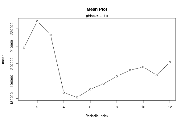
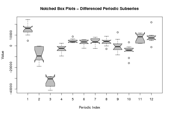
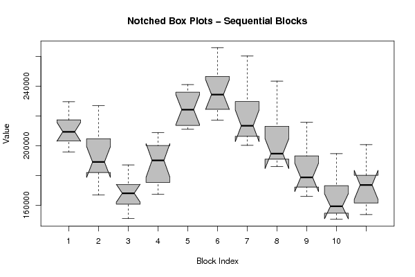
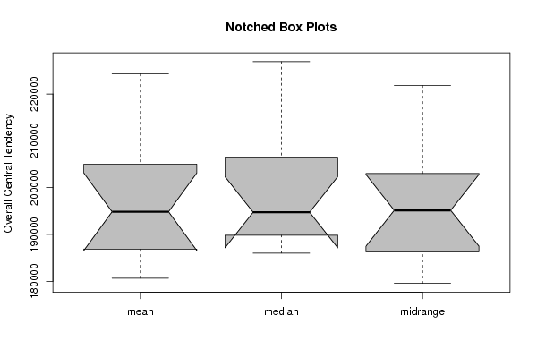
| Title produced by software | Mean Plot | ||||||||||||||||||||
| Date of computation | Fri, 17 Dec 2010 13:44:39 +0000 | ||||||||||||||||||||
| Cite this page as follows | Statistical Computations at FreeStatistics.org, Office for Research Development and Education, URL https://freestatistics.org/blog/index.php?v=date/2010/Dec/17/t1292593379900ret6x84mxmro.htm/, Retrieved Tue, 16 Sep 2025 13:34:52 +0000 | ||||||||||||||||||||
| Statistical Computations at FreeStatistics.org, Office for Research Development and Education, URL https://freestatistics.org/blog/index.php?pk=111461, Retrieved Tue, 16 Sep 2025 13:34:52 +0000 | |||||||||||||||||||||
| QR Codes: | |||||||||||||||||||||
|
| |||||||||||||||||||||
| Original text written by user: | |||||||||||||||||||||
| IsPrivate? | No (this computation is public) | ||||||||||||||||||||
| User-defined keywords | |||||||||||||||||||||
| Estimated Impact | 293 | ||||||||||||||||||||
Tree of Dependent Computations | |||||||||||||||||||||
| Family? (F = Feedback message, R = changed R code, M = changed R Module, P = changed Parameters, D = changed Data) | |||||||||||||||||||||
| - [Bivariate Data Series] [Bivariate dataset] [2008-01-05 23:51:08] [74be16979710d4c4e7c6647856088456] F RMPD [Mean Plot] [Colombia Coffee] [2008-01-07 13:38:24] [74be16979710d4c4e7c6647856088456] - MPD [Mean Plot] [Retailprijs - Sei...] [2010-11-05 10:26:46] [aeb27d5c05332f2e597ad139ee63fbe4] - D [Mean Plot] [Mean Plot - Niet ...] [2010-11-12 11:43:04] [aeb27d5c05332f2e597ad139ee63fbe4] - D [Mean Plot] [Mean Plot – Nie...] [2010-12-17 13:44:39] [18ef3d986e8801a4b28404e69e5bf56b] [Current] | |||||||||||||||||||||
| Feedback Forum | |||||||||||||||||||||
Post a new message | |||||||||||||||||||||
Dataset | |||||||||||||||||||||
| Dataseries X: | |||||||||||||||||||||
211868 229527 229139 198563 195722 202196 205816 212588 214320 220375 204442 206903 214126 226899 223532 195309 186005 188906 191563 189226 186413 178037 166827 169362 174330 187069 186530 158114 151001 159612 161914 164182 169701 171297 166444 173476 182516 202388 202300 168053 167302 172608 178106 185686 194581 194596 197922 208795 230580 240636 240048 211457 211142 214771 212610 219313 219277 231805 229245 241114 248624 265845 256446 219452 217142 221678 227184 230354 235243 237217 233575 244460 243324 260307 241476 203666 200237 204045 209465 213586 216234 213188 208679 217859 227247 243477 232571 191531 186029 189733 190420 194163 198770 195198 193111 195411 202108 215706 206348 166972 166070 169292 175041 177876 181140 179566 175335 184128 189917 194690 179612 150605 150569 153745 155511 159044 163095 159585 158644 166618 176512 200765 182698 153730 156145 161570 165688 173666 180144 | |||||||||||||||||||||
Tables (Output of Computation) | |||||||||||||||||||||
| |||||||||||||||||||||
Figures (Output of Computation) | |||||||||||||||||||||
Input Parameters & R Code | |||||||||||||||||||||
| Parameters (Session): | |||||||||||||||||||||
| par1 = 12 ; | |||||||||||||||||||||
| Parameters (R input): | |||||||||||||||||||||
| par1 = 12 ; | |||||||||||||||||||||
| R code (references can be found in the software module): | |||||||||||||||||||||
par1 <- as.numeric(par1) | |||||||||||||||||||||