Repository of Reproducible Computations

Free Statistics

of Irreproducible Research!

Author's title

Author

*The author of this computation has been verified*

R Software Module

rwasp_autocorrelation.wasp

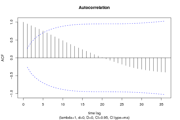
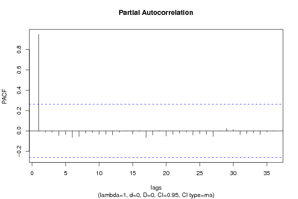
Title produced by software

(Partial) Autocorrelation Function

Date of computation

Fri, 17 Dec 2010 12:15:05 +0000

Cite this page as follows

Statistical Computations at FreeStatistics.org, Office for Research Development and Education, URL https://freestatistics.org/blog/index.php?v=date/2010/Dec/17/t129258799555bi3qj95s3n9m4.htm/, Retrieved Wed, 01 May 2024 20:45:21 +0000

Statistical Computations at FreeStatistics.org, Office for Research Development and Education, URL https://freestatistics.org/blog/index.php?pk=111418, Retrieved Wed, 01 May 2024 20:45:21 +0000

QR Codes:

Paste this QR Code to cite your computation.

Original text written by user:

IsPrivate?

No (this computation is public)

User-defined keywords

Estimated Impact

176

Family? (F = Feedback message, R = changed R code, M = changed R Module, P = changed Parameters, D = changed Data)

-     [Univariate Explorative Data Analysis] [Run Sequence gebo...] [2008-12-12 13:32:37] [76963dc1903f0f612b6153510a3818cf]
- R  D  [Univariate Explorative Data Analysis] [Run Sequence gebo...] [2008-12-17 12:14:40] [76963dc1903f0f612b6153510a3818cf]
-         [Univariate Explorative Data Analysis] [Run Sequence Plot...] [2008-12-22 18:19:51] [1ce0d16c8f4225c977b42c8fa93bc163]
- RMP       [(Partial) Autocorrelation Function] [Identifying Integ...] [2009-11-22 12:16:10] [b98453cac15ba1066b407e146608df68]
-    D        [(Partial) Autocorrelation Function] [Model 1 (d = 0, D...] [2009-11-24 17:27:24] [ee7c2e7343f5b1451e62c5c16ec521f1]
-    D          [(Partial) Autocorrelation Function] [Methode 1 (D=0, d=0)] [2009-11-27 12:01:23] [76ab39dc7a55316678260825bd5ad46c]
-    D            [(Partial) Autocorrelation Function] [methode 1 (d=0 D= 0)] [2009-11-27 20:21:42] [4b453aa14d54730625f8d3de5f1f6d82]
-    D              [(Partial) Autocorrelation Function] [koffie en thee] [2009-12-16 19:04:55] [7773f496f69461f4a67891f0ef752622]
-    D                [(Partial) Autocorrelation Function] [Appelen Jonagold ...] [2009-12-17 16:51:16] [7773f496f69461f4a67891f0ef752622]
-    D                  [(Partial) Autocorrelation Function] [biefstuk 3] [2010-12-14 15:31:38] [3df61981e9f4dafed65341be376c4457]
- R  D                      [(Partial) Autocorrelation Function] [restaurant 2] [2010-12-17 12:15:05] [6e52d1bada9435d33ddf990b22ee4b00] [Current]
-   PD                        [(Partial) Autocorrelation Function] [restaurant 3] [2010-12-17 12:25:43] [3df61981e9f4dafed65341be376c4457] 

Feedback Forum

Post a new message

Dataseries X:

Download CSV

Histogram

Boxplots

Summary of computational transaction
Raw Input	view raw input (R code)
Raw Output	view raw output of R engine
Computing time	2 seconds
R Server	'George Udny Yule' @ 72.249.76.132

\begin{tabular}{lllllllll}
\hline
Summary of computational transaction \tabularnewline
Raw Input & view raw input (R code)  \tabularnewline
Raw Output & view raw output of R engine  \tabularnewline
Computing time & 2 seconds \tabularnewline
R Server & 'George Udny Yule' @ 72.249.76.132 \tabularnewline
\hline
\end{tabular}
%Source: https://freestatistics.org/blog/index.php?pk=111418&T=0

[TABLE]
[ROW][C]Summary of computational transaction[/C][/ROW]
[ROW][C]Raw Input[/C][C]view raw input (R code) [/C][/ROW]
[ROW][C]Raw Output[/C][C]view raw output of R engine [/C][/ROW]
[ROW][C]Computing time[/C][C]2 seconds[/C][/ROW]
[ROW][C]R Server[/C][C]'George Udny Yule' @ 72.249.76.132[/C][/ROW]
[/TABLE]
Source: https://freestatistics.org/blog/index.php?pk=111418&T=0

Globally Unique Identifier (entire table): ba.freestatistics.org/blog/index.php?pk=111418&T=0

As an alternative you can also use a QR Code:

The GUIDs for individual cells are displayed in the table below:

Summary of computational transaction
Raw Input	view raw input (R code)
Raw Output	view raw output of R engine
Computing time	2 seconds
R Server	'George Udny Yule' @ 72.249.76.132

Autocorrelation Function
Time lag k	ACF(k)	T-STAT	P-value
1	0.950243	7.111	0
2	0.901777	6.7483	0
3	0.854515	6.3946	0
4	0.805077	6.0246	0
5	0.75477	5.6482	0
6	0.701133	5.2468	1e-06
7	0.645241	4.8285	6e-06
8	0.590584	4.4195	2.3e-05
9	0.53759	4.023	8.7e-05
10	0.484436	3.6252	0.000312
11	0.431405	3.2283	0.001042
12	0.37793	2.8282	0.003242
13	0.326975	2.4469	0.008787
14	0.279451	2.0912	0.020529
15	0.232423	1.7393	0.043738
16	0.188395	1.4098	0.082062
17	0.141732	1.0606	0.146707
18	0.09538	0.7138	0.23917
19	0.053869	0.4031	0.344199
20	0.011246	0.0842	0.466614
21	-0.030768	-0.2302	0.409369
22	-0.070937	-0.5308	0.298814
23	-0.108188	-0.8096	0.210797
24	-0.145149	-1.0862	0.141022
25	-0.180241	-1.3488	0.091416
26	-0.214424	-1.6046	0.057103
27	-0.249453	-1.8667	0.033589
28	-0.279745	-2.0934	0.020426
29	-0.303202	-2.269	0.013572
30	-0.321374	-2.4049	0.009753
31	-0.339772	-2.5426	0.006897
32	-0.356816	-2.6702	0.004952
33	-0.371509	-2.7801	0.003693
34	-0.385514	-2.8849	0.002774
35	-0.395955	-2.9631	0.002233
36	-0.403231	-3.0175	0.001915

\begin{tabular}{lllllllll}
\hline
Autocorrelation Function \tabularnewline
Time lag k & ACF(k) & T-STAT & P-value \tabularnewline
1 & 0.950243 & 7.111 & 0 \tabularnewline
2 & 0.901777 & 6.7483 & 0 \tabularnewline
3 & 0.854515 & 6.3946 & 0 \tabularnewline
4 & 0.805077 & 6.0246 & 0 \tabularnewline
5 & 0.75477 & 5.6482 & 0 \tabularnewline
6 & 0.701133 & 5.2468 & 1e-06 \tabularnewline
7 & 0.645241 & 4.8285 & 6e-06 \tabularnewline
8 & 0.590584 & 4.4195 & 2.3e-05 \tabularnewline
9 & 0.53759 & 4.023 & 8.7e-05 \tabularnewline
10 & 0.484436 & 3.6252 & 0.000312 \tabularnewline
11 & 0.431405 & 3.2283 & 0.001042 \tabularnewline
12 & 0.37793 & 2.8282 & 0.003242 \tabularnewline
13 & 0.326975 & 2.4469 & 0.008787 \tabularnewline
14 & 0.279451 & 2.0912 & 0.020529 \tabularnewline
15 & 0.232423 & 1.7393 & 0.043738 \tabularnewline
16 & 0.188395 & 1.4098 & 0.082062 \tabularnewline
17 & 0.141732 & 1.0606 & 0.146707 \tabularnewline
18 & 0.09538 & 0.7138 & 0.23917 \tabularnewline
19 & 0.053869 & 0.4031 & 0.344199 \tabularnewline
20 & 0.011246 & 0.0842 & 0.466614 \tabularnewline
21 & -0.030768 & -0.2302 & 0.409369 \tabularnewline
22 & -0.070937 & -0.5308 & 0.298814 \tabularnewline
23 & -0.108188 & -0.8096 & 0.210797 \tabularnewline
24 & -0.145149 & -1.0862 & 0.141022 \tabularnewline
25 & -0.180241 & -1.3488 & 0.091416 \tabularnewline
26 & -0.214424 & -1.6046 & 0.057103 \tabularnewline
27 & -0.249453 & -1.8667 & 0.033589 \tabularnewline
28 & -0.279745 & -2.0934 & 0.020426 \tabularnewline
29 & -0.303202 & -2.269 & 0.013572 \tabularnewline
30 & -0.321374 & -2.4049 & 0.009753 \tabularnewline
31 & -0.339772 & -2.5426 & 0.006897 \tabularnewline
32 & -0.356816 & -2.6702 & 0.004952 \tabularnewline
33 & -0.371509 & -2.7801 & 0.003693 \tabularnewline
34 & -0.385514 & -2.8849 & 0.002774 \tabularnewline
35 & -0.395955 & -2.9631 & 0.002233 \tabularnewline
36 & -0.403231 & -3.0175 & 0.001915 \tabularnewline
\hline
\end{tabular}
%Source: https://freestatistics.org/blog/index.php?pk=111418&T=1

[TABLE]
[ROW][C]Autocorrelation Function[/C][/ROW]
[ROW][C]Time lag k[/C][C]ACF(k)[/C][C]T-STAT[/C][C]P-value[/C][/ROW]
[ROW][C]1[/C][C]0.950243[/C][C]7.111[/C][C]0[/C][/ROW]
[ROW][C]2[/C][C]0.901777[/C][C]6.7483[/C][C]0[/C][/ROW]
[ROW][C]3[/C][C]0.854515[/C][C]6.3946[/C][C]0[/C][/ROW]
[ROW][C]4[/C][C]0.805077[/C][C]6.0246[/C][C]0[/C][/ROW]
[ROW][C]5[/C][C]0.75477[/C][C]5.6482[/C][C]0[/C][/ROW]
[ROW][C]6[/C][C]0.701133[/C][C]5.2468[/C][C]1e-06[/C][/ROW]
[ROW][C]7[/C][C]0.645241[/C][C]4.8285[/C][C]6e-06[/C][/ROW]
[ROW][C]8[/C][C]0.590584[/C][C]4.4195[/C][C]2.3e-05[/C][/ROW]
[ROW][C]9[/C][C]0.53759[/C][C]4.023[/C][C]8.7e-05[/C][/ROW]
[ROW][C]10[/C][C]0.484436[/C][C]3.6252[/C][C]0.000312[/C][/ROW]
[ROW][C]11[/C][C]0.431405[/C][C]3.2283[/C][C]0.001042[/C][/ROW]
[ROW][C]12[/C][C]0.37793[/C][C]2.8282[/C][C]0.003242[/C][/ROW]
[ROW][C]13[/C][C]0.326975[/C][C]2.4469[/C][C]0.008787[/C][/ROW]
[ROW][C]14[/C][C]0.279451[/C][C]2.0912[/C][C]0.020529[/C][/ROW]
[ROW][C]15[/C][C]0.232423[/C][C]1.7393[/C][C]0.043738[/C][/ROW]
[ROW][C]16[/C][C]0.188395[/C][C]1.4098[/C][C]0.082062[/C][/ROW]
[ROW][C]17[/C][C]0.141732[/C][C]1.0606[/C][C]0.146707[/C][/ROW]
[ROW][C]18[/C][C]0.09538[/C][C]0.7138[/C][C]0.23917[/C][/ROW]
[ROW][C]19[/C][C]0.053869[/C][C]0.4031[/C][C]0.344199[/C][/ROW]
[ROW][C]20[/C][C]0.011246[/C][C]0.0842[/C][C]0.466614[/C][/ROW]
[ROW][C]21[/C][C]-0.030768[/C][C]-0.2302[/C][C]0.409369[/C][/ROW]
[ROW][C]22[/C][C]-0.070937[/C][C]-0.5308[/C][C]0.298814[/C][/ROW]
[ROW][C]23[/C][C]-0.108188[/C][C]-0.8096[/C][C]0.210797[/C][/ROW]
[ROW][C]24[/C][C]-0.145149[/C][C]-1.0862[/C][C]0.141022[/C][/ROW]
[ROW][C]25[/C][C]-0.180241[/C][C]-1.3488[/C][C]0.091416[/C][/ROW]
[ROW][C]26[/C][C]-0.214424[/C][C]-1.6046[/C][C]0.057103[/C][/ROW]
[ROW][C]27[/C][C]-0.249453[/C][C]-1.8667[/C][C]0.033589[/C][/ROW]
[ROW][C]28[/C][C]-0.279745[/C][C]-2.0934[/C][C]0.020426[/C][/ROW]
[ROW][C]29[/C][C]-0.303202[/C][C]-2.269[/C][C]0.013572[/C][/ROW]
[ROW][C]30[/C][C]-0.321374[/C][C]-2.4049[/C][C]0.009753[/C][/ROW]
[ROW][C]31[/C][C]-0.339772[/C][C]-2.5426[/C][C]0.006897[/C][/ROW]
[ROW][C]32[/C][C]-0.356816[/C][C]-2.6702[/C][C]0.004952[/C][/ROW]
[ROW][C]33[/C][C]-0.371509[/C][C]-2.7801[/C][C]0.003693[/C][/ROW]
[ROW][C]34[/C][C]-0.385514[/C][C]-2.8849[/C][C]0.002774[/C][/ROW]
[ROW][C]35[/C][C]-0.395955[/C][C]-2.9631[/C][C]0.002233[/C][/ROW]
[ROW][C]36[/C][C]-0.403231[/C][C]-3.0175[/C][C]0.001915[/C][/ROW]
[/TABLE]
Source: https://freestatistics.org/blog/index.php?pk=111418&T=1

Globally Unique Identifier (entire table): ba.freestatistics.org/blog/index.php?pk=111418&T=1

As an alternative you can also use a QR Code:

The GUIDs for individual cells are displayed in the table below:

Autocorrelation Function
Time lag k	ACF(k)	T-STAT	P-value
1	0.950243	7.111	0
2	0.901777	6.7483	0
3	0.854515	6.3946	0
4	0.805077	6.0246	0
5	0.75477	5.6482	0
6	0.701133	5.2468	1e-06
7	0.645241	4.8285	6e-06
8	0.590584	4.4195	2.3e-05
9	0.53759	4.023	8.7e-05
10	0.484436	3.6252	0.000312
11	0.431405	3.2283	0.001042
12	0.37793	2.8282	0.003242
13	0.326975	2.4469	0.008787
14	0.279451	2.0912	0.020529
15	0.232423	1.7393	0.043738
16	0.188395	1.4098	0.082062
17	0.141732	1.0606	0.146707
18	0.09538	0.7138	0.23917
19	0.053869	0.4031	0.344199
20	0.011246	0.0842	0.466614
21	-0.030768	-0.2302	0.409369
22	-0.070937	-0.5308	0.298814
23	-0.108188	-0.8096	0.210797
24	-0.145149	-1.0862	0.141022
25	-0.180241	-1.3488	0.091416
26	-0.214424	-1.6046	0.057103
27	-0.249453	-1.8667	0.033589
28	-0.279745	-2.0934	0.020426
29	-0.303202	-2.269	0.013572
30	-0.321374	-2.4049	0.009753
31	-0.339772	-2.5426	0.006897
32	-0.356816	-2.6702	0.004952
33	-0.371509	-2.7801	0.003693
34	-0.385514	-2.8849	0.002774
35	-0.395955	-2.9631	0.002233
36	-0.403231	-3.0175	0.001915

Partial Autocorrelation Function
Time lag k	PACF(k)	T-STAT	P-value
1	0.950243	7.111	0
2	-0.012216	-0.0914	0.463745
3	-0.012915	-0.0966	0.461675
4	-0.047606	-0.3563	0.361495
5	-0.036773	-0.2752	0.392095
6	-0.06389	-0.4781	0.317217
7	-0.05576	-0.4173	0.339037
8	-0.022571	-0.1689	0.43324
9	-0.015997	-0.1197	0.452572
10	-0.033809	-0.253	0.400597
11	-0.03301	-0.247	0.402897
12	-0.04097	-0.3066	0.380145
13	-0.012999	-0.0973	0.461429
14	-0.003564	-0.0267	0.48941
15	-0.030718	-0.2299	0.409514
16	-0.006339	-0.0474	0.481167
17	-0.065199	-0.4879	0.31376
18	-0.040027	-0.2995	0.38282
19	0.002787	0.0209	0.491719
20	-0.051686	-0.3868	0.350192
21	-0.036062	-0.2699	0.394129
22	-0.025448	-0.1904	0.424827
23	-0.011634	-0.0871	0.465468
24	-0.042401	-0.3173	0.376097
25	-0.027981	-0.2094	0.417452
26	-0.034569	-0.2587	0.398411
27	-0.055331	-0.4141	0.340207
28	-0.001973	-0.0148	0.494137
29	0.025155	0.1882	0.425683
30	0.014582	0.1091	0.456748
31	-0.038031	-0.2846	0.388501
32	-0.028185	-0.2109	0.416859
33	-0.021403	-0.1602	0.436663
34	-0.037659	-0.2818	0.389562
35	-0.011343	-0.0849	0.466329
36	-0.003617	-0.0271	0.489253

\begin{tabular}{lllllllll}
\hline
Partial Autocorrelation Function \tabularnewline
Time lag k & PACF(k) & T-STAT & P-value \tabularnewline
1 & 0.950243 & 7.111 & 0 \tabularnewline
2 & -0.012216 & -0.0914 & 0.463745 \tabularnewline
3 & -0.012915 & -0.0966 & 0.461675 \tabularnewline
4 & -0.047606 & -0.3563 & 0.361495 \tabularnewline
5 & -0.036773 & -0.2752 & 0.392095 \tabularnewline
6 & -0.06389 & -0.4781 & 0.317217 \tabularnewline
7 & -0.05576 & -0.4173 & 0.339037 \tabularnewline
8 & -0.022571 & -0.1689 & 0.43324 \tabularnewline
9 & -0.015997 & -0.1197 & 0.452572 \tabularnewline
10 & -0.033809 & -0.253 & 0.400597 \tabularnewline
11 & -0.03301 & -0.247 & 0.402897 \tabularnewline
12 & -0.04097 & -0.3066 & 0.380145 \tabularnewline
13 & -0.012999 & -0.0973 & 0.461429 \tabularnewline
14 & -0.003564 & -0.0267 & 0.48941 \tabularnewline
15 & -0.030718 & -0.2299 & 0.409514 \tabularnewline
16 & -0.006339 & -0.0474 & 0.481167 \tabularnewline
17 & -0.065199 & -0.4879 & 0.31376 \tabularnewline
18 & -0.040027 & -0.2995 & 0.38282 \tabularnewline
19 & 0.002787 & 0.0209 & 0.491719 \tabularnewline
20 & -0.051686 & -0.3868 & 0.350192 \tabularnewline
21 & -0.036062 & -0.2699 & 0.394129 \tabularnewline
22 & -0.025448 & -0.1904 & 0.424827 \tabularnewline
23 & -0.011634 & -0.0871 & 0.465468 \tabularnewline
24 & -0.042401 & -0.3173 & 0.376097 \tabularnewline
25 & -0.027981 & -0.2094 & 0.417452 \tabularnewline
26 & -0.034569 & -0.2587 & 0.398411 \tabularnewline
27 & -0.055331 & -0.4141 & 0.340207 \tabularnewline
28 & -0.001973 & -0.0148 & 0.494137 \tabularnewline
29 & 0.025155 & 0.1882 & 0.425683 \tabularnewline
30 & 0.014582 & 0.1091 & 0.456748 \tabularnewline
31 & -0.038031 & -0.2846 & 0.388501 \tabularnewline
32 & -0.028185 & -0.2109 & 0.416859 \tabularnewline
33 & -0.021403 & -0.1602 & 0.436663 \tabularnewline
34 & -0.037659 & -0.2818 & 0.389562 \tabularnewline
35 & -0.011343 & -0.0849 & 0.466329 \tabularnewline
36 & -0.003617 & -0.0271 & 0.489253 \tabularnewline
\hline
\end{tabular}
%Source: https://freestatistics.org/blog/index.php?pk=111418&T=2

[TABLE]
[ROW][C]Partial Autocorrelation Function[/C][/ROW]
[ROW][C]Time lag k[/C][C]PACF(k)[/C][C]T-STAT[/C][C]P-value[/C][/ROW]
[ROW][C]1[/C][C]0.950243[/C][C]7.111[/C][C]0[/C][/ROW]
[ROW][C]2[/C][C]-0.012216[/C][C]-0.0914[/C][C]0.463745[/C][/ROW]
[ROW][C]3[/C][C]-0.012915[/C][C]-0.0966[/C][C]0.461675[/C][/ROW]
[ROW][C]4[/C][C]-0.047606[/C][C]-0.3563[/C][C]0.361495[/C][/ROW]
[ROW][C]5[/C][C]-0.036773[/C][C]-0.2752[/C][C]0.392095[/C][/ROW]
[ROW][C]6[/C][C]-0.06389[/C][C]-0.4781[/C][C]0.317217[/C][/ROW]
[ROW][C]7[/C][C]-0.05576[/C][C]-0.4173[/C][C]0.339037[/C][/ROW]
[ROW][C]8[/C][C]-0.022571[/C][C]-0.1689[/C][C]0.43324[/C][/ROW]
[ROW][C]9[/C][C]-0.015997[/C][C]-0.1197[/C][C]0.452572[/C][/ROW]
[ROW][C]10[/C][C]-0.033809[/C][C]-0.253[/C][C]0.400597[/C][/ROW]
[ROW][C]11[/C][C]-0.03301[/C][C]-0.247[/C][C]0.402897[/C][/ROW]
[ROW][C]12[/C][C]-0.04097[/C][C]-0.3066[/C][C]0.380145[/C][/ROW]
[ROW][C]13[/C][C]-0.012999[/C][C]-0.0973[/C][C]0.461429[/C][/ROW]
[ROW][C]14[/C][C]-0.003564[/C][C]-0.0267[/C][C]0.48941[/C][/ROW]
[ROW][C]15[/C][C]-0.030718[/C][C]-0.2299[/C][C]0.409514[/C][/ROW]
[ROW][C]16[/C][C]-0.006339[/C][C]-0.0474[/C][C]0.481167[/C][/ROW]
[ROW][C]17[/C][C]-0.065199[/C][C]-0.4879[/C][C]0.31376[/C][/ROW]
[ROW][C]18[/C][C]-0.040027[/C][C]-0.2995[/C][C]0.38282[/C][/ROW]
[ROW][C]19[/C][C]0.002787[/C][C]0.0209[/C][C]0.491719[/C][/ROW]
[ROW][C]20[/C][C]-0.051686[/C][C]-0.3868[/C][C]0.350192[/C][/ROW]
[ROW][C]21[/C][C]-0.036062[/C][C]-0.2699[/C][C]0.394129[/C][/ROW]
[ROW][C]22[/C][C]-0.025448[/C][C]-0.1904[/C][C]0.424827[/C][/ROW]
[ROW][C]23[/C][C]-0.011634[/C][C]-0.0871[/C][C]0.465468[/C][/ROW]
[ROW][C]24[/C][C]-0.042401[/C][C]-0.3173[/C][C]0.376097[/C][/ROW]
[ROW][C]25[/C][C]-0.027981[/C][C]-0.2094[/C][C]0.417452[/C][/ROW]
[ROW][C]26[/C][C]-0.034569[/C][C]-0.2587[/C][C]0.398411[/C][/ROW]
[ROW][C]27[/C][C]-0.055331[/C][C]-0.4141[/C][C]0.340207[/C][/ROW]
[ROW][C]28[/C][C]-0.001973[/C][C]-0.0148[/C][C]0.494137[/C][/ROW]
[ROW][C]29[/C][C]0.025155[/C][C]0.1882[/C][C]0.425683[/C][/ROW]
[ROW][C]30[/C][C]0.014582[/C][C]0.1091[/C][C]0.456748[/C][/ROW]
[ROW][C]31[/C][C]-0.038031[/C][C]-0.2846[/C][C]0.388501[/C][/ROW]
[ROW][C]32[/C][C]-0.028185[/C][C]-0.2109[/C][C]0.416859[/C][/ROW]
[ROW][C]33[/C][C]-0.021403[/C][C]-0.1602[/C][C]0.436663[/C][/ROW]
[ROW][C]34[/C][C]-0.037659[/C][C]-0.2818[/C][C]0.389562[/C][/ROW]
[ROW][C]35[/C][C]-0.011343[/C][C]-0.0849[/C][C]0.466329[/C][/ROW]
[ROW][C]36[/C][C]-0.003617[/C][C]-0.0271[/C][C]0.489253[/C][/ROW]
[/TABLE]
Source: https://freestatistics.org/blog/index.php?pk=111418&T=2

Globally Unique Identifier (entire table): ba.freestatistics.org/blog/index.php?pk=111418&T=2

As an alternative you can also use a QR Code:

The GUIDs for individual cells are displayed in the table below:

Partial Autocorrelation Function
Time lag k	PACF(k)	T-STAT	P-value
1	0.950243	7.111	0
2	-0.012216	-0.0914	0.463745
3	-0.012915	-0.0966	0.461675
4	-0.047606	-0.3563	0.361495
5	-0.036773	-0.2752	0.392095
6	-0.06389	-0.4781	0.317217
7	-0.05576	-0.4173	0.339037
8	-0.022571	-0.1689	0.43324
9	-0.015997	-0.1197	0.452572
10	-0.033809	-0.253	0.400597
11	-0.03301	-0.247	0.402897
12	-0.04097	-0.3066	0.380145
13	-0.012999	-0.0973	0.461429
14	-0.003564	-0.0267	0.48941
15	-0.030718	-0.2299	0.409514
16	-0.006339	-0.0474	0.481167
17	-0.065199	-0.4879	0.31376
18	-0.040027	-0.2995	0.38282
19	0.002787	0.0209	0.491719
20	-0.051686	-0.3868	0.350192
21	-0.036062	-0.2699	0.394129
22	-0.025448	-0.1904	0.424827
23	-0.011634	-0.0871	0.465468
24	-0.042401	-0.3173	0.376097
25	-0.027981	-0.2094	0.417452
26	-0.034569	-0.2587	0.398411
27	-0.055331	-0.4141	0.340207
28	-0.001973	-0.0148	0.494137
29	0.025155	0.1882	0.425683
30	0.014582	0.1091	0.456748
31	-0.038031	-0.2846	0.388501
32	-0.028185	-0.2109	0.416859
33	-0.021403	-0.1602	0.436663
34	-0.037659	-0.2818	0.389562
35	-0.011343	-0.0849	0.466329
36	-0.003617	-0.0271	0.489253

Figure 1

PNG link

Postscript link

PDF link

Figure 2

PNG link

Postscript link

PDF link

Figure 3

PNG link

Postscript link

PDF link

Parameters (Session):

par1 = 36 ; par2 = 1 ; par3 = 0 ; par4 = 0 ; par5 = 12 ; par6 = MA ; par7 = 0.95 ;

Parameters (R input):

par1 = 36 ; par2 = 1 ; par3 = 0 ; par4 = 0 ; par5 = 12 ; par6 = MA ; par7 = 0.95 ; par8 = ;

R code (references can be found in the software module):

if (par1 == 'Default') {
par1 = 10*log10(length(x))
} else {
par1 <- as.numeric(par1)
}
par2 <- as.numeric(par2)
par3 <- as.numeric(par3)
par4 <- as.numeric(par4)
par5 <- as.numeric(par5)
if (par6 == 'White Noise') par6 <- 'white' else par6 <- 'ma'
par7 <- as.numeric(par7)
if (par8 != '') par8 <- as.numeric(par8)
ox <- x
if (par8 == '') {
if (par2 == 0) {
x <- log(x)
} else {
x <- (x ^ par2 - 1) / par2
}
} else {
x <- log(x,base=par8)
}
if (par3 > 0) x <- diff(x,lag=1,difference=par3)
if (par4 > 0) x <- diff(x,lag=par5,difference=par4)
bitmap(file='picts.png')
op <- par(mfrow=c(2,1))
plot(ox,type='l',main='Original Time Series',xlab='time',ylab='value')
if (par8=='') {
mytitle <- paste('Working Time Series (lambda=',par2,', d=',par3,', D=',par4,')',sep='')
mysub <- paste('(lambda=',par2,', d=',par3,', D=',par4,', CI=', par7, ', CI type=',par6,')',sep='')
} else {
mytitle <- paste('Working Time Series (base=',par8,', d=',par3,', D=',par4,')',sep='')
mysub <- paste('(base=',par8,', d=',par3,', D=',par4,', CI=', par7, ', CI type=',par6,')',sep='')
}
plot(x,type='l', main=mytitle,xlab='time',ylab='value')
par(op)
dev.off()
bitmap(file='pic1.png')
racf <- acf(x, par1, main='Autocorrelation', xlab='time lag', ylab='ACF', ci.type=par6, ci=par7, sub=mysub)
dev.off()
bitmap(file='pic2.png')
rpacf <- pacf(x,par1,main='Partial Autocorrelation',xlab='lags',ylab='PACF',sub=mysub)
dev.off()
(myacf <- c(racf$acf))
(mypacf <- c(rpacf$acf))
lengthx <- length(x)
sqrtn <- sqrt(lengthx)
load(file='createtable')
a<-table.start()
a<-table.row.start(a)
a<-table.element(a,'Autocorrelation Function',4,TRUE)
a<-table.row.end(a)
a<-table.row.start(a)
a<-table.element(a,'Time lag k',header=TRUE)
a<-table.element(a,hyperlink('basics.htm','ACF(k)','click here for more information about the Autocorrelation Function'),header=TRUE)
a<-table.element(a,'T-STAT',header=TRUE)
a<-table.element(a,'P-value',header=TRUE)
a<-table.row.end(a)
for (i in 2:(par1+1)) {
a<-table.row.start(a)
a<-table.element(a,i-1,header=TRUE)
a<-table.element(a,round(myacf[i],6))
mytstat <- myacf[i]*sqrtn
a<-table.element(a,round(mytstat,4))
a<-table.element(a,round(1-pt(abs(mytstat),lengthx),6))
a<-table.row.end(a)
}
a<-table.end(a)
table.save(a,file='mytable.tab')
a<-table.start()
a<-table.row.start(a)
a<-table.element(a,'Partial Autocorrelation Function',4,TRUE)
a<-table.row.end(a)
a<-table.row.start(a)
a<-table.element(a,'Time lag k',header=TRUE)
a<-table.element(a,hyperlink('basics.htm','PACF(k)','click here for more information about the Partial Autocorrelation Function'),header=TRUE)
a<-table.element(a,'T-STAT',header=TRUE)
a<-table.element(a,'P-value',header=TRUE)
a<-table.row.end(a)
for (i in 1:par1) {
a<-table.row.start(a)
a<-table.element(a,i,header=TRUE)
a<-table.element(a,round(mypacf[i],6))
mytstat <- mypacf[i]*sqrtn
a<-table.element(a,round(mytstat,4))
a<-table.element(a,round(1-pt(abs(mytstat),lengthx),6))
a<-table.row.end(a)
}
a<-table.end(a)
table.save(a,file='mytable1.tab')

Free Statistics

Description of Statistical Computation

Tree of Dependent Computations

Dataset

Tables (Output of Computation)

Figures (Output of Computation)

Input Parameters & R Code