Repository of Reproducible Computations

Free Statistics

of Irreproducible Research!

Author's title

Author

*The author of this computation has been verified*

R Software Module

rwasp_autocorrelation.wasp

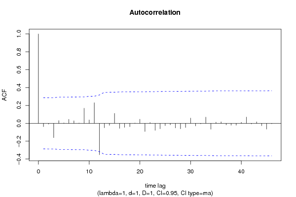
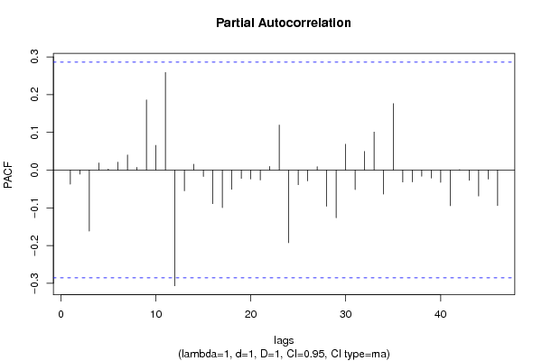
Title produced by software

(Partial) Autocorrelation Function

Date of computation

Wed, 15 Dec 2010 16:55:24 +0000

Cite this page as follows

Statistical Computations at FreeStatistics.org, Office for Research Development and Education, URL https://freestatistics.org/blog/index.php?v=date/2010/Dec/15/t1292431986o6y4k9v2eg23i6o.htm/, Retrieved Wed, 01 May 2024 14:09:36 +0000

Statistical Computations at FreeStatistics.org, Office for Research Development and Education, URL https://freestatistics.org/blog/index.php?pk=110572, Retrieved Wed, 01 May 2024 14:09:36 +0000

QR Codes:

Paste this QR Code to cite your computation.

Original text written by user:

IsPrivate?

No (this computation is public)

User-defined keywords

Estimated Impact

165

Family? (F = Feedback message, R = changed R code, M = changed R Module, P = changed Parameters, D = changed Data)

-     [Univariate Explorative Data Analysis] [Run Sequence gebo...] [2008-12-12 13:32:37] [76963dc1903f0f612b6153510a3818cf]
- R  D  [Univariate Explorative Data Analysis] [Run Sequence gebo...] [2008-12-17 12:14:40] [76963dc1903f0f612b6153510a3818cf]
-         [Univariate Explorative Data Analysis] [Run Sequence Plot...] [2008-12-22 18:19:51] [1ce0d16c8f4225c977b42c8fa93bc163]
- RMP       [(Partial) Autocorrelation Function] [Identifying Integ...] [2009-11-22 12:16:10] [b98453cac15ba1066b407e146608df68]
-    D        [(Partial) Autocorrelation Function] [Model 1 (d = 0, D...] [2009-11-24 17:27:24] [ee7c2e7343f5b1451e62c5c16ec521f1]
-    D          [(Partial) Autocorrelation Function] [Methode 1 (D=0, d=0)] [2009-11-27 12:01:23] [76ab39dc7a55316678260825bd5ad46c]
-    D            [(Partial) Autocorrelation Function] [methode 1 (d=0 D= 0)] [2009-11-27 20:21:42] [4b453aa14d54730625f8d3de5f1f6d82]
-    D              [(Partial) Autocorrelation Function] [koffie en thee] [2009-12-16 19:04:55] [7773f496f69461f4a67891f0ef752622]
-    D                [(Partial) Autocorrelation Function] [Appelen Jonagold ...] [2009-12-17 16:51:16] [7773f496f69461f4a67891f0ef752622]
- R PD                    [(Partial) Autocorrelation Function] [autocorrelatie] [2010-12-15 16:55:24] [c1f1b5e209adb4577289f490325e36f2] [Current]
-   P                       [(Partial) Autocorrelation Function] [autocorrelatie] [2010-12-18 09:15:00] [717f3d787904f94c39256c5c1fc72d4c] 

Feedback Forum

Post a new message

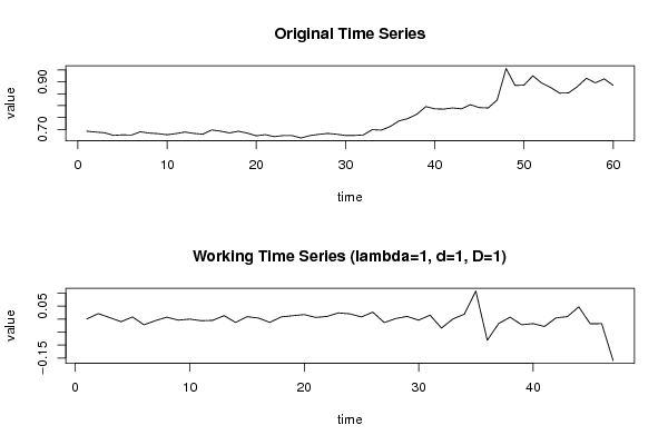
Dataseries X:

Download CSV

Histogram

Boxplots

Summary of computational transaction
Raw Input	view raw input (R code)
Raw Output	view raw output of R engine
Computing time	2 seconds
R Server	'George Udny Yule' @ 72.249.76.132

\begin{tabular}{lllllllll}
\hline
Summary of computational transaction \tabularnewline
Raw Input & view raw input (R code)  \tabularnewline
Raw Output & view raw output of R engine  \tabularnewline
Computing time & 2 seconds \tabularnewline
R Server & 'George Udny Yule' @ 72.249.76.132 \tabularnewline
\hline
\end{tabular}
%Source: https://freestatistics.org/blog/index.php?pk=110572&T=0

[TABLE]
[ROW][C]Summary of computational transaction[/C][/ROW]
[ROW][C]Raw Input[/C][C]view raw input (R code) [/C][/ROW]
[ROW][C]Raw Output[/C][C]view raw output of R engine [/C][/ROW]
[ROW][C]Computing time[/C][C]2 seconds[/C][/ROW]
[ROW][C]R Server[/C][C]'George Udny Yule' @ 72.249.76.132[/C][/ROW]
[/TABLE]
Source: https://freestatistics.org/blog/index.php?pk=110572&T=0

Globally Unique Identifier (entire table): ba.freestatistics.org/blog/index.php?pk=110572&T=0

As an alternative you can also use a QR Code:

The GUIDs for individual cells are displayed in the table below:

Summary of computational transaction
Raw Input	view raw input (R code)
Raw Output	view raw output of R engine
Computing time	2 seconds
R Server	'George Udny Yule' @ 72.249.76.132

Autocorrelation Function
Time lag k	ACF(k)	T-STAT	P-value
1	-0.037291	-0.2557	0.399666
2	-0.009273	-0.0636	0.47479
3	-0.160711	-1.1018	0.138084
4	0.030776	0.211	0.416903
5	0.00505	0.0346	0.486265
6	0.045358	0.311	0.378603
7	0.02861	0.1961	0.422674
8	0.00289	0.0198	0.492138
9	0.168616	1.156	0.126768
10	0.038586	0.2645	0.396262
11	0.230336	1.5791	0.06051
12	-0.351639	-2.4107	0.009943
13	-0.049998	-0.3428	0.366649
14	-0.023149	-0.1587	0.437292
15	0.111027	0.7612	0.225181
16	-0.056961	-0.3905	0.348965
17	-0.045968	-0.3151	0.377024
18	-0.038293	-0.2625	0.397033
19	0.003377	0.0232	0.490814
20	0.045814	0.3141	0.377423
21	-0.091777	-0.6292	0.266135
22	0.009411	0.0645	0.474416
23	-0.07916	-0.5427	0.294952
24	-0.061586	-0.4222	0.337398
25	-0.026426	-0.1812	0.428507
26	-0.016981	-0.1164	0.453908
27	-0.052201	-0.3579	0.36102
28	-0.061351	-0.4206	0.337981
29	-0.04727	-0.3241	0.373662
30	0.059219	0.406	0.343299
31	-0.030059	-0.2061	0.418812
32	-0.005877	-0.0403	0.484017
33	0.069183	0.4743	0.318744
34	-0.06625	-0.4542	0.325893
35	0.013048	0.0895	0.46455
36	0.017272	0.1184	0.453123
37	-0.018285	-0.1254	0.450389
38	-0.021389	-0.1466	0.442025
39	-0.021378	-0.1466	0.442052
40	0.011634	0.0798	0.468385
41	0.070074	0.4804	0.316583
42	-0.007151	-0.049	0.480553
43	0.017265	0.1184	0.453142
44	-0.027421	-0.188	0.425848
45	-0.064793	-0.4442	0.329468
46	-0.004908	-0.0336	0.486651
47	NA	NA	NA
48	NA	NA	NA
49	NA	NA	NA
50	NA	NA	NA
51	NA	NA	NA
52	NA	NA	NA
53	NA	NA	NA
54	NA	NA	NA
55	NA	NA	NA
56	NA	NA	NA
57	NA	NA	NA
58	NA	NA	NA
59	NA	NA	NA
60	NA	NA	NA

\begin{tabular}{lllllllll}
\hline
Autocorrelation Function \tabularnewline
Time lag k & ACF(k) & T-STAT & P-value \tabularnewline
1 & -0.037291 & -0.2557 & 0.399666 \tabularnewline
2 & -0.009273 & -0.0636 & 0.47479 \tabularnewline
3 & -0.160711 & -1.1018 & 0.138084 \tabularnewline
4 & 0.030776 & 0.211 & 0.416903 \tabularnewline
5 & 0.00505 & 0.0346 & 0.486265 \tabularnewline
6 & 0.045358 & 0.311 & 0.378603 \tabularnewline
7 & 0.02861 & 0.1961 & 0.422674 \tabularnewline
8 & 0.00289 & 0.0198 & 0.492138 \tabularnewline
9 & 0.168616 & 1.156 & 0.126768 \tabularnewline
10 & 0.038586 & 0.2645 & 0.396262 \tabularnewline
11 & 0.230336 & 1.5791 & 0.06051 \tabularnewline
12 & -0.351639 & -2.4107 & 0.009943 \tabularnewline
13 & -0.049998 & -0.3428 & 0.366649 \tabularnewline
14 & -0.023149 & -0.1587 & 0.437292 \tabularnewline
15 & 0.111027 & 0.7612 & 0.225181 \tabularnewline
16 & -0.056961 & -0.3905 & 0.348965 \tabularnewline
17 & -0.045968 & -0.3151 & 0.377024 \tabularnewline
18 & -0.038293 & -0.2625 & 0.397033 \tabularnewline
19 & 0.003377 & 0.0232 & 0.490814 \tabularnewline
20 & 0.045814 & 0.3141 & 0.377423 \tabularnewline
21 & -0.091777 & -0.6292 & 0.266135 \tabularnewline
22 & 0.009411 & 0.0645 & 0.474416 \tabularnewline
23 & -0.07916 & -0.5427 & 0.294952 \tabularnewline
24 & -0.061586 & -0.4222 & 0.337398 \tabularnewline
25 & -0.026426 & -0.1812 & 0.428507 \tabularnewline
26 & -0.016981 & -0.1164 & 0.453908 \tabularnewline
27 & -0.052201 & -0.3579 & 0.36102 \tabularnewline
28 & -0.061351 & -0.4206 & 0.337981 \tabularnewline
29 & -0.04727 & -0.3241 & 0.373662 \tabularnewline
30 & 0.059219 & 0.406 & 0.343299 \tabularnewline
31 & -0.030059 & -0.2061 & 0.418812 \tabularnewline
32 & -0.005877 & -0.0403 & 0.484017 \tabularnewline
33 & 0.069183 & 0.4743 & 0.318744 \tabularnewline
34 & -0.06625 & -0.4542 & 0.325893 \tabularnewline
35 & 0.013048 & 0.0895 & 0.46455 \tabularnewline
36 & 0.017272 & 0.1184 & 0.453123 \tabularnewline
37 & -0.018285 & -0.1254 & 0.450389 \tabularnewline
38 & -0.021389 & -0.1466 & 0.442025 \tabularnewline
39 & -0.021378 & -0.1466 & 0.442052 \tabularnewline
40 & 0.011634 & 0.0798 & 0.468385 \tabularnewline
41 & 0.070074 & 0.4804 & 0.316583 \tabularnewline
42 & -0.007151 & -0.049 & 0.480553 \tabularnewline
43 & 0.017265 & 0.1184 & 0.453142 \tabularnewline
44 & -0.027421 & -0.188 & 0.425848 \tabularnewline
45 & -0.064793 & -0.4442 & 0.329468 \tabularnewline
46 & -0.004908 & -0.0336 & 0.486651 \tabularnewline
47 & NA & NA & NA \tabularnewline
48 & NA & NA & NA \tabularnewline
49 & NA & NA & NA \tabularnewline
50 & NA & NA & NA \tabularnewline
51 & NA & NA & NA \tabularnewline
52 & NA & NA & NA \tabularnewline
53 & NA & NA & NA \tabularnewline
54 & NA & NA & NA \tabularnewline
55 & NA & NA & NA \tabularnewline
56 & NA & NA & NA \tabularnewline
57 & NA & NA & NA \tabularnewline
58 & NA & NA & NA \tabularnewline
59 & NA & NA & NA \tabularnewline
60 & NA & NA & NA \tabularnewline
\hline
\end{tabular}
%Source: https://freestatistics.org/blog/index.php?pk=110572&T=1

[TABLE]
[ROW][C]Autocorrelation Function[/C][/ROW]
[ROW][C]Time lag k[/C][C]ACF(k)[/C][C]T-STAT[/C][C]P-value[/C][/ROW]
[ROW][C]1[/C][C]-0.037291[/C][C]-0.2557[/C][C]0.399666[/C][/ROW]
[ROW][C]2[/C][C]-0.009273[/C][C]-0.0636[/C][C]0.47479[/C][/ROW]
[ROW][C]3[/C][C]-0.160711[/C][C]-1.1018[/C][C]0.138084[/C][/ROW]
[ROW][C]4[/C][C]0.030776[/C][C]0.211[/C][C]0.416903[/C][/ROW]
[ROW][C]5[/C][C]0.00505[/C][C]0.0346[/C][C]0.486265[/C][/ROW]
[ROW][C]6[/C][C]0.045358[/C][C]0.311[/C][C]0.378603[/C][/ROW]
[ROW][C]7[/C][C]0.02861[/C][C]0.1961[/C][C]0.422674[/C][/ROW]
[ROW][C]8[/C][C]0.00289[/C][C]0.0198[/C][C]0.492138[/C][/ROW]
[ROW][C]9[/C][C]0.168616[/C][C]1.156[/C][C]0.126768[/C][/ROW]
[ROW][C]10[/C][C]0.038586[/C][C]0.2645[/C][C]0.396262[/C][/ROW]
[ROW][C]11[/C][C]0.230336[/C][C]1.5791[/C][C]0.06051[/C][/ROW]
[ROW][C]12[/C][C]-0.351639[/C][C]-2.4107[/C][C]0.009943[/C][/ROW]
[ROW][C]13[/C][C]-0.049998[/C][C]-0.3428[/C][C]0.366649[/C][/ROW]
[ROW][C]14[/C][C]-0.023149[/C][C]-0.1587[/C][C]0.437292[/C][/ROW]
[ROW][C]15[/C][C]0.111027[/C][C]0.7612[/C][C]0.225181[/C][/ROW]
[ROW][C]16[/C][C]-0.056961[/C][C]-0.3905[/C][C]0.348965[/C][/ROW]
[ROW][C]17[/C][C]-0.045968[/C][C]-0.3151[/C][C]0.377024[/C][/ROW]
[ROW][C]18[/C][C]-0.038293[/C][C]-0.2625[/C][C]0.397033[/C][/ROW]
[ROW][C]19[/C][C]0.003377[/C][C]0.0232[/C][C]0.490814[/C][/ROW]
[ROW][C]20[/C][C]0.045814[/C][C]0.3141[/C][C]0.377423[/C][/ROW]
[ROW][C]21[/C][C]-0.091777[/C][C]-0.6292[/C][C]0.266135[/C][/ROW]
[ROW][C]22[/C][C]0.009411[/C][C]0.0645[/C][C]0.474416[/C][/ROW]
[ROW][C]23[/C][C]-0.07916[/C][C]-0.5427[/C][C]0.294952[/C][/ROW]
[ROW][C]24[/C][C]-0.061586[/C][C]-0.4222[/C][C]0.337398[/C][/ROW]
[ROW][C]25[/C][C]-0.026426[/C][C]-0.1812[/C][C]0.428507[/C][/ROW]
[ROW][C]26[/C][C]-0.016981[/C][C]-0.1164[/C][C]0.453908[/C][/ROW]
[ROW][C]27[/C][C]-0.052201[/C][C]-0.3579[/C][C]0.36102[/C][/ROW]
[ROW][C]28[/C][C]-0.061351[/C][C]-0.4206[/C][C]0.337981[/C][/ROW]
[ROW][C]29[/C][C]-0.04727[/C][C]-0.3241[/C][C]0.373662[/C][/ROW]
[ROW][C]30[/C][C]0.059219[/C][C]0.406[/C][C]0.343299[/C][/ROW]
[ROW][C]31[/C][C]-0.030059[/C][C]-0.2061[/C][C]0.418812[/C][/ROW]
[ROW][C]32[/C][C]-0.005877[/C][C]-0.0403[/C][C]0.484017[/C][/ROW]
[ROW][C]33[/C][C]0.069183[/C][C]0.4743[/C][C]0.318744[/C][/ROW]
[ROW][C]34[/C][C]-0.06625[/C][C]-0.4542[/C][C]0.325893[/C][/ROW]
[ROW][C]35[/C][C]0.013048[/C][C]0.0895[/C][C]0.46455[/C][/ROW]
[ROW][C]36[/C][C]0.017272[/C][C]0.1184[/C][C]0.453123[/C][/ROW]
[ROW][C]37[/C][C]-0.018285[/C][C]-0.1254[/C][C]0.450389[/C][/ROW]
[ROW][C]38[/C][C]-0.021389[/C][C]-0.1466[/C][C]0.442025[/C][/ROW]
[ROW][C]39[/C][C]-0.021378[/C][C]-0.1466[/C][C]0.442052[/C][/ROW]
[ROW][C]40[/C][C]0.011634[/C][C]0.0798[/C][C]0.468385[/C][/ROW]
[ROW][C]41[/C][C]0.070074[/C][C]0.4804[/C][C]0.316583[/C][/ROW]
[ROW][C]42[/C][C]-0.007151[/C][C]-0.049[/C][C]0.480553[/C][/ROW]
[ROW][C]43[/C][C]0.017265[/C][C]0.1184[/C][C]0.453142[/C][/ROW]
[ROW][C]44[/C][C]-0.027421[/C][C]-0.188[/C][C]0.425848[/C][/ROW]
[ROW][C]45[/C][C]-0.064793[/C][C]-0.4442[/C][C]0.329468[/C][/ROW]
[ROW][C]46[/C][C]-0.004908[/C][C]-0.0336[/C][C]0.486651[/C][/ROW]
[ROW][C]47[/C][C]NA[/C][C]NA[/C][C]NA[/C][/ROW]
[ROW][C]48[/C][C]NA[/C][C]NA[/C][C]NA[/C][/ROW]
[ROW][C]49[/C][C]NA[/C][C]NA[/C][C]NA[/C][/ROW]
[ROW][C]50[/C][C]NA[/C][C]NA[/C][C]NA[/C][/ROW]
[ROW][C]51[/C][C]NA[/C][C]NA[/C][C]NA[/C][/ROW]
[ROW][C]52[/C][C]NA[/C][C]NA[/C][C]NA[/C][/ROW]
[ROW][C]53[/C][C]NA[/C][C]NA[/C][C]NA[/C][/ROW]
[ROW][C]54[/C][C]NA[/C][C]NA[/C][C]NA[/C][/ROW]
[ROW][C]55[/C][C]NA[/C][C]NA[/C][C]NA[/C][/ROW]
[ROW][C]56[/C][C]NA[/C][C]NA[/C][C]NA[/C][/ROW]
[ROW][C]57[/C][C]NA[/C][C]NA[/C][C]NA[/C][/ROW]
[ROW][C]58[/C][C]NA[/C][C]NA[/C][C]NA[/C][/ROW]
[ROW][C]59[/C][C]NA[/C][C]NA[/C][C]NA[/C][/ROW]
[ROW][C]60[/C][C]NA[/C][C]NA[/C][C]NA[/C][/ROW]
[/TABLE]
Source: https://freestatistics.org/blog/index.php?pk=110572&T=1

Globally Unique Identifier (entire table): ba.freestatistics.org/blog/index.php?pk=110572&T=1

As an alternative you can also use a QR Code:

The GUIDs for individual cells are displayed in the table below:

Autocorrelation Function
Time lag k	ACF(k)	T-STAT	P-value
1	-0.037291	-0.2557	0.399666
2	-0.009273	-0.0636	0.47479
3	-0.160711	-1.1018	0.138084
4	0.030776	0.211	0.416903
5	0.00505	0.0346	0.486265
6	0.045358	0.311	0.378603
7	0.02861	0.1961	0.422674
8	0.00289	0.0198	0.492138
9	0.168616	1.156	0.126768
10	0.038586	0.2645	0.396262
11	0.230336	1.5791	0.06051
12	-0.351639	-2.4107	0.009943
13	-0.049998	-0.3428	0.366649
14	-0.023149	-0.1587	0.437292
15	0.111027	0.7612	0.225181
16	-0.056961	-0.3905	0.348965
17	-0.045968	-0.3151	0.377024
18	-0.038293	-0.2625	0.397033
19	0.003377	0.0232	0.490814
20	0.045814	0.3141	0.377423
21	-0.091777	-0.6292	0.266135
22	0.009411	0.0645	0.474416
23	-0.07916	-0.5427	0.294952
24	-0.061586	-0.4222	0.337398
25	-0.026426	-0.1812	0.428507
26	-0.016981	-0.1164	0.453908
27	-0.052201	-0.3579	0.36102
28	-0.061351	-0.4206	0.337981
29	-0.04727	-0.3241	0.373662
30	0.059219	0.406	0.343299
31	-0.030059	-0.2061	0.418812
32	-0.005877	-0.0403	0.484017
33	0.069183	0.4743	0.318744
34	-0.06625	-0.4542	0.325893
35	0.013048	0.0895	0.46455
36	0.017272	0.1184	0.453123
37	-0.018285	-0.1254	0.450389
38	-0.021389	-0.1466	0.442025
39	-0.021378	-0.1466	0.442052
40	0.011634	0.0798	0.468385
41	0.070074	0.4804	0.316583
42	-0.007151	-0.049	0.480553
43	0.017265	0.1184	0.453142
44	-0.027421	-0.188	0.425848
45	-0.064793	-0.4442	0.329468
46	-0.004908	-0.0336	0.486651
47	NA	NA	NA
48	NA	NA	NA
49	NA	NA	NA
50	NA	NA	NA
51	NA	NA	NA
52	NA	NA	NA
53	NA	NA	NA
54	NA	NA	NA
55	NA	NA	NA
56	NA	NA	NA
57	NA	NA	NA
58	NA	NA	NA
59	NA	NA	NA
60	NA	NA	NA

Partial Autocorrelation Function
Time lag k	PACF(k)	T-STAT	P-value
1	-0.037291	-0.2557	0.399666
2	-0.010678	-0.0732	0.470976
3	-0.161702	-1.1086	0.136628
4	0.018775	0.1287	0.449067
5	0.00281	0.0193	0.492355
6	0.021042	0.1443	0.442957
7	0.040244	0.2759	0.391917
8	0.007332	0.0503	0.480061
9	0.185959	1.2749	0.104311
10	0.065407	0.4484	0.327959
11	0.258706	1.7736	0.041304
12	-0.30666	-2.1024	0.020453
13	-0.055072	-0.3776	0.353732
14	0.015549	0.1066	0.457781
15	-0.016903	-0.1159	0.45412
16	-0.08916	-0.6113	0.271989
17	-0.099438	-0.6817	0.249384
18	-0.051197	-0.351	0.363583
19	-0.022125	-0.1517	0.440044
20	-0.023661	-0.1622	0.435917
21	-0.026205	-0.1797	0.429099
22	0.009749	0.0668	0.473498
23	0.119257	0.8176	0.20886
24	-0.192513	-1.3198	0.096647
25	-0.038722	-0.2655	0.395907
26	-0.028763	-0.1972	0.422265
27	0.009051	0.0621	0.475392
28	-0.095825	-0.6569	0.257211
29	-0.126298	-0.8659	0.195484
30	0.068494	0.4696	0.320416
31	-0.051752	-0.3548	0.362165
32	0.049453	0.339	0.368048
33	0.100821	0.6912	0.246422
34	-0.0637	-0.4367	0.332164
35	0.176034	1.2068	0.116768
36	-0.031774	-0.2178	0.414251
37	-0.031231	-0.2141	0.415693
38	-0.016367	-0.1122	0.455569
39	-0.021222	-0.1455	0.442472
40	-0.032577	-0.2233	0.412122
41	-0.094291	-0.6464	0.260573
42	0.001188	0.0081	0.496769
43	-0.027205	-0.1865	0.426425
44	-0.068779	-0.4715	0.319723
45	-0.023813	-0.1633	0.43551
46	-0.094005	-0.6445	0.261202
47	NA	NA	NA
48	NA	NA	NA
49	NA	NA	NA
50	NA	NA	NA
51	NA	NA	NA
52	NA	NA	NA
53	NA	NA	NA
54	NA	NA	NA
55	NA	NA	NA
56	NA	NA	NA
57	NA	NA	NA
58	NA	NA	NA
59	NA	NA	NA
60	NA	NA	NA

\begin{tabular}{lllllllll}
\hline
Partial Autocorrelation Function \tabularnewline
Time lag k & PACF(k) & T-STAT & P-value \tabularnewline
1 & -0.037291 & -0.2557 & 0.399666 \tabularnewline
2 & -0.010678 & -0.0732 & 0.470976 \tabularnewline
3 & -0.161702 & -1.1086 & 0.136628 \tabularnewline
4 & 0.018775 & 0.1287 & 0.449067 \tabularnewline
5 & 0.00281 & 0.0193 & 0.492355 \tabularnewline
6 & 0.021042 & 0.1443 & 0.442957 \tabularnewline
7 & 0.040244 & 0.2759 & 0.391917 \tabularnewline
8 & 0.007332 & 0.0503 & 0.480061 \tabularnewline
9 & 0.185959 & 1.2749 & 0.104311 \tabularnewline
10 & 0.065407 & 0.4484 & 0.327959 \tabularnewline
11 & 0.258706 & 1.7736 & 0.041304 \tabularnewline
12 & -0.30666 & -2.1024 & 0.020453 \tabularnewline
13 & -0.055072 & -0.3776 & 0.353732 \tabularnewline
14 & 0.015549 & 0.1066 & 0.457781 \tabularnewline
15 & -0.016903 & -0.1159 & 0.45412 \tabularnewline
16 & -0.08916 & -0.6113 & 0.271989 \tabularnewline
17 & -0.099438 & -0.6817 & 0.249384 \tabularnewline
18 & -0.051197 & -0.351 & 0.363583 \tabularnewline
19 & -0.022125 & -0.1517 & 0.440044 \tabularnewline
20 & -0.023661 & -0.1622 & 0.435917 \tabularnewline
21 & -0.026205 & -0.1797 & 0.429099 \tabularnewline
22 & 0.009749 & 0.0668 & 0.473498 \tabularnewline
23 & 0.119257 & 0.8176 & 0.20886 \tabularnewline
24 & -0.192513 & -1.3198 & 0.096647 \tabularnewline
25 & -0.038722 & -0.2655 & 0.395907 \tabularnewline
26 & -0.028763 & -0.1972 & 0.422265 \tabularnewline
27 & 0.009051 & 0.0621 & 0.475392 \tabularnewline
28 & -0.095825 & -0.6569 & 0.257211 \tabularnewline
29 & -0.126298 & -0.8659 & 0.195484 \tabularnewline
30 & 0.068494 & 0.4696 & 0.320416 \tabularnewline
31 & -0.051752 & -0.3548 & 0.362165 \tabularnewline
32 & 0.049453 & 0.339 & 0.368048 \tabularnewline
33 & 0.100821 & 0.6912 & 0.246422 \tabularnewline
34 & -0.0637 & -0.4367 & 0.332164 \tabularnewline
35 & 0.176034 & 1.2068 & 0.116768 \tabularnewline
36 & -0.031774 & -0.2178 & 0.414251 \tabularnewline
37 & -0.031231 & -0.2141 & 0.415693 \tabularnewline
38 & -0.016367 & -0.1122 & 0.455569 \tabularnewline
39 & -0.021222 & -0.1455 & 0.442472 \tabularnewline
40 & -0.032577 & -0.2233 & 0.412122 \tabularnewline
41 & -0.094291 & -0.6464 & 0.260573 \tabularnewline
42 & 0.001188 & 0.0081 & 0.496769 \tabularnewline
43 & -0.027205 & -0.1865 & 0.426425 \tabularnewline
44 & -0.068779 & -0.4715 & 0.319723 \tabularnewline
45 & -0.023813 & -0.1633 & 0.43551 \tabularnewline
46 & -0.094005 & -0.6445 & 0.261202 \tabularnewline
47 & NA & NA & NA \tabularnewline
48 & NA & NA & NA \tabularnewline
49 & NA & NA & NA \tabularnewline
50 & NA & NA & NA \tabularnewline
51 & NA & NA & NA \tabularnewline
52 & NA & NA & NA \tabularnewline
53 & NA & NA & NA \tabularnewline
54 & NA & NA & NA \tabularnewline
55 & NA & NA & NA \tabularnewline
56 & NA & NA & NA \tabularnewline
57 & NA & NA & NA \tabularnewline
58 & NA & NA & NA \tabularnewline
59 & NA & NA & NA \tabularnewline
60 & NA & NA & NA \tabularnewline
\hline
\end{tabular}
%Source: https://freestatistics.org/blog/index.php?pk=110572&T=2

[TABLE]
[ROW][C]Partial Autocorrelation Function[/C][/ROW]
[ROW][C]Time lag k[/C][C]PACF(k)[/C][C]T-STAT[/C][C]P-value[/C][/ROW]
[ROW][C]1[/C][C]-0.037291[/C][C]-0.2557[/C][C]0.399666[/C][/ROW]
[ROW][C]2[/C][C]-0.010678[/C][C]-0.0732[/C][C]0.470976[/C][/ROW]
[ROW][C]3[/C][C]-0.161702[/C][C]-1.1086[/C][C]0.136628[/C][/ROW]
[ROW][C]4[/C][C]0.018775[/C][C]0.1287[/C][C]0.449067[/C][/ROW]
[ROW][C]5[/C][C]0.00281[/C][C]0.0193[/C][C]0.492355[/C][/ROW]
[ROW][C]6[/C][C]0.021042[/C][C]0.1443[/C][C]0.442957[/C][/ROW]
[ROW][C]7[/C][C]0.040244[/C][C]0.2759[/C][C]0.391917[/C][/ROW]
[ROW][C]8[/C][C]0.007332[/C][C]0.0503[/C][C]0.480061[/C][/ROW]
[ROW][C]9[/C][C]0.185959[/C][C]1.2749[/C][C]0.104311[/C][/ROW]
[ROW][C]10[/C][C]0.065407[/C][C]0.4484[/C][C]0.327959[/C][/ROW]
[ROW][C]11[/C][C]0.258706[/C][C]1.7736[/C][C]0.041304[/C][/ROW]
[ROW][C]12[/C][C]-0.30666[/C][C]-2.1024[/C][C]0.020453[/C][/ROW]
[ROW][C]13[/C][C]-0.055072[/C][C]-0.3776[/C][C]0.353732[/C][/ROW]
[ROW][C]14[/C][C]0.015549[/C][C]0.1066[/C][C]0.457781[/C][/ROW]
[ROW][C]15[/C][C]-0.016903[/C][C]-0.1159[/C][C]0.45412[/C][/ROW]
[ROW][C]16[/C][C]-0.08916[/C][C]-0.6113[/C][C]0.271989[/C][/ROW]
[ROW][C]17[/C][C]-0.099438[/C][C]-0.6817[/C][C]0.249384[/C][/ROW]
[ROW][C]18[/C][C]-0.051197[/C][C]-0.351[/C][C]0.363583[/C][/ROW]
[ROW][C]19[/C][C]-0.022125[/C][C]-0.1517[/C][C]0.440044[/C][/ROW]
[ROW][C]20[/C][C]-0.023661[/C][C]-0.1622[/C][C]0.435917[/C][/ROW]
[ROW][C]21[/C][C]-0.026205[/C][C]-0.1797[/C][C]0.429099[/C][/ROW]
[ROW][C]22[/C][C]0.009749[/C][C]0.0668[/C][C]0.473498[/C][/ROW]
[ROW][C]23[/C][C]0.119257[/C][C]0.8176[/C][C]0.20886[/C][/ROW]
[ROW][C]24[/C][C]-0.192513[/C][C]-1.3198[/C][C]0.096647[/C][/ROW]
[ROW][C]25[/C][C]-0.038722[/C][C]-0.2655[/C][C]0.395907[/C][/ROW]
[ROW][C]26[/C][C]-0.028763[/C][C]-0.1972[/C][C]0.422265[/C][/ROW]
[ROW][C]27[/C][C]0.009051[/C][C]0.0621[/C][C]0.475392[/C][/ROW]
[ROW][C]28[/C][C]-0.095825[/C][C]-0.6569[/C][C]0.257211[/C][/ROW]
[ROW][C]29[/C][C]-0.126298[/C][C]-0.8659[/C][C]0.195484[/C][/ROW]
[ROW][C]30[/C][C]0.068494[/C][C]0.4696[/C][C]0.320416[/C][/ROW]
[ROW][C]31[/C][C]-0.051752[/C][C]-0.3548[/C][C]0.362165[/C][/ROW]
[ROW][C]32[/C][C]0.049453[/C][C]0.339[/C][C]0.368048[/C][/ROW]
[ROW][C]33[/C][C]0.100821[/C][C]0.6912[/C][C]0.246422[/C][/ROW]
[ROW][C]34[/C][C]-0.0637[/C][C]-0.4367[/C][C]0.332164[/C][/ROW]
[ROW][C]35[/C][C]0.176034[/C][C]1.2068[/C][C]0.116768[/C][/ROW]
[ROW][C]36[/C][C]-0.031774[/C][C]-0.2178[/C][C]0.414251[/C][/ROW]
[ROW][C]37[/C][C]-0.031231[/C][C]-0.2141[/C][C]0.415693[/C][/ROW]
[ROW][C]38[/C][C]-0.016367[/C][C]-0.1122[/C][C]0.455569[/C][/ROW]
[ROW][C]39[/C][C]-0.021222[/C][C]-0.1455[/C][C]0.442472[/C][/ROW]
[ROW][C]40[/C][C]-0.032577[/C][C]-0.2233[/C][C]0.412122[/C][/ROW]
[ROW][C]41[/C][C]-0.094291[/C][C]-0.6464[/C][C]0.260573[/C][/ROW]
[ROW][C]42[/C][C]0.001188[/C][C]0.0081[/C][C]0.496769[/C][/ROW]
[ROW][C]43[/C][C]-0.027205[/C][C]-0.1865[/C][C]0.426425[/C][/ROW]
[ROW][C]44[/C][C]-0.068779[/C][C]-0.4715[/C][C]0.319723[/C][/ROW]
[ROW][C]45[/C][C]-0.023813[/C][C]-0.1633[/C][C]0.43551[/C][/ROW]
[ROW][C]46[/C][C]-0.094005[/C][C]-0.6445[/C][C]0.261202[/C][/ROW]
[ROW][C]47[/C][C]NA[/C][C]NA[/C][C]NA[/C][/ROW]
[ROW][C]48[/C][C]NA[/C][C]NA[/C][C]NA[/C][/ROW]
[ROW][C]49[/C][C]NA[/C][C]NA[/C][C]NA[/C][/ROW]
[ROW][C]50[/C][C]NA[/C][C]NA[/C][C]NA[/C][/ROW]
[ROW][C]51[/C][C]NA[/C][C]NA[/C][C]NA[/C][/ROW]
[ROW][C]52[/C][C]NA[/C][C]NA[/C][C]NA[/C][/ROW]
[ROW][C]53[/C][C]NA[/C][C]NA[/C][C]NA[/C][/ROW]
[ROW][C]54[/C][C]NA[/C][C]NA[/C][C]NA[/C][/ROW]
[ROW][C]55[/C][C]NA[/C][C]NA[/C][C]NA[/C][/ROW]
[ROW][C]56[/C][C]NA[/C][C]NA[/C][C]NA[/C][/ROW]
[ROW][C]57[/C][C]NA[/C][C]NA[/C][C]NA[/C][/ROW]
[ROW][C]58[/C][C]NA[/C][C]NA[/C][C]NA[/C][/ROW]
[ROW][C]59[/C][C]NA[/C][C]NA[/C][C]NA[/C][/ROW]
[ROW][C]60[/C][C]NA[/C][C]NA[/C][C]NA[/C][/ROW]
[/TABLE]
Source: https://freestatistics.org/blog/index.php?pk=110572&T=2

Globally Unique Identifier (entire table): ba.freestatistics.org/blog/index.php?pk=110572&T=2

As an alternative you can also use a QR Code:

The GUIDs for individual cells are displayed in the table below:

Partial Autocorrelation Function
Time lag k	PACF(k)	T-STAT	P-value
1	-0.037291	-0.2557	0.399666
2	-0.010678	-0.0732	0.470976
3	-0.161702	-1.1086	0.136628
4	0.018775	0.1287	0.449067
5	0.00281	0.0193	0.492355
6	0.021042	0.1443	0.442957
7	0.040244	0.2759	0.391917
8	0.007332	0.0503	0.480061
9	0.185959	1.2749	0.104311
10	0.065407	0.4484	0.327959
11	0.258706	1.7736	0.041304
12	-0.30666	-2.1024	0.020453
13	-0.055072	-0.3776	0.353732
14	0.015549	0.1066	0.457781
15	-0.016903	-0.1159	0.45412
16	-0.08916	-0.6113	0.271989
17	-0.099438	-0.6817	0.249384
18	-0.051197	-0.351	0.363583
19	-0.022125	-0.1517	0.440044
20	-0.023661	-0.1622	0.435917
21	-0.026205	-0.1797	0.429099
22	0.009749	0.0668	0.473498
23	0.119257	0.8176	0.20886
24	-0.192513	-1.3198	0.096647
25	-0.038722	-0.2655	0.395907
26	-0.028763	-0.1972	0.422265
27	0.009051	0.0621	0.475392
28	-0.095825	-0.6569	0.257211
29	-0.126298	-0.8659	0.195484
30	0.068494	0.4696	0.320416
31	-0.051752	-0.3548	0.362165
32	0.049453	0.339	0.368048
33	0.100821	0.6912	0.246422
34	-0.0637	-0.4367	0.332164
35	0.176034	1.2068	0.116768
36	-0.031774	-0.2178	0.414251
37	-0.031231	-0.2141	0.415693
38	-0.016367	-0.1122	0.455569
39	-0.021222	-0.1455	0.442472
40	-0.032577	-0.2233	0.412122
41	-0.094291	-0.6464	0.260573
42	0.001188	0.0081	0.496769
43	-0.027205	-0.1865	0.426425
44	-0.068779	-0.4715	0.319723
45	-0.023813	-0.1633	0.43551
46	-0.094005	-0.6445	0.261202
47	NA	NA	NA
48	NA	NA	NA
49	NA	NA	NA
50	NA	NA	NA
51	NA	NA	NA
52	NA	NA	NA
53	NA	NA	NA
54	NA	NA	NA
55	NA	NA	NA
56	NA	NA	NA
57	NA	NA	NA
58	NA	NA	NA
59	NA	NA	NA
60	NA	NA	NA

Figure 1

PNG link

Postscript link

PDF link

Figure 2

PNG link

Postscript link

PDF link

Figure 3

PNG link

Postscript link

PDF link

Parameters (Session):

par1 = 1 ; par2 = 0 ; par3 = 0 ; par4 = 12 ; par5 = 1 ; par6 = 0 ; par7 = 0 ;

Parameters (R input):

par1 = 60 ; par2 = 1 ; par3 = 1 ; par4 = 1 ; par5 = 12 ; par6 = MA ; par7 = 0.95 ; par8 = ;

R code (references can be found in the software module):

if (par1 == 'Default') {
par1 = 10*log10(length(x))
} else {
par1 <- as.numeric(par1)
}
par2 <- as.numeric(par2)
par3 <- as.numeric(par3)
par4 <- as.numeric(par4)
par5 <- as.numeric(par5)
if (par6 == 'White Noise') par6 <- 'white' else par6 <- 'ma'
par7 <- as.numeric(par7)
if (par8 != '') par8 <- as.numeric(par8)
ox <- x
if (par8 == '') {
if (par2 == 0) {
x <- log(x)
} else {
x <- (x ^ par2 - 1) / par2
}
} else {
x <- log(x,base=par8)
}
if (par3 > 0) x <- diff(x,lag=1,difference=par3)
if (par4 > 0) x <- diff(x,lag=par5,difference=par4)
bitmap(file='picts.png')
op <- par(mfrow=c(2,1))
plot(ox,type='l',main='Original Time Series',xlab='time',ylab='value')
if (par8=='') {
mytitle <- paste('Working Time Series (lambda=',par2,', d=',par3,', D=',par4,')',sep='')
mysub <- paste('(lambda=',par2,', d=',par3,', D=',par4,', CI=', par7, ', CI type=',par6,')',sep='')
} else {
mytitle <- paste('Working Time Series (base=',par8,', d=',par3,', D=',par4,')',sep='')
mysub <- paste('(base=',par8,', d=',par3,', D=',par4,', CI=', par7, ', CI type=',par6,')',sep='')
}
plot(x,type='l', main=mytitle,xlab='time',ylab='value')
par(op)
dev.off()
bitmap(file='pic1.png')
racf <- acf(x, par1, main='Autocorrelation', xlab='time lag', ylab='ACF', ci.type=par6, ci=par7, sub=mysub)
dev.off()
bitmap(file='pic2.png')
rpacf <- pacf(x,par1,main='Partial Autocorrelation',xlab='lags',ylab='PACF',sub=mysub)
dev.off()
(myacf <- c(racf$acf))
(mypacf <- c(rpacf$acf))
lengthx <- length(x)
sqrtn <- sqrt(lengthx)
load(file='createtable')
a<-table.start()
a<-table.row.start(a)
a<-table.element(a,'Autocorrelation Function',4,TRUE)
a<-table.row.end(a)
a<-table.row.start(a)
a<-table.element(a,'Time lag k',header=TRUE)
a<-table.element(a,hyperlink('basics.htm','ACF(k)','click here for more information about the Autocorrelation Function'),header=TRUE)
a<-table.element(a,'T-STAT',header=TRUE)
a<-table.element(a,'P-value',header=TRUE)
a<-table.row.end(a)
for (i in 2:(par1+1)) {
a<-table.row.start(a)
a<-table.element(a,i-1,header=TRUE)
a<-table.element(a,round(myacf[i],6))
mytstat <- myacf[i]*sqrtn
a<-table.element(a,round(mytstat,4))
a<-table.element(a,round(1-pt(abs(mytstat),lengthx),6))
a<-table.row.end(a)
}
a<-table.end(a)
table.save(a,file='mytable.tab')
a<-table.start()
a<-table.row.start(a)
a<-table.element(a,'Partial Autocorrelation Function',4,TRUE)
a<-table.row.end(a)
a<-table.row.start(a)
a<-table.element(a,'Time lag k',header=TRUE)
a<-table.element(a,hyperlink('basics.htm','PACF(k)','click here for more information about the Partial Autocorrelation Function'),header=TRUE)
a<-table.element(a,'T-STAT',header=TRUE)
a<-table.element(a,'P-value',header=TRUE)
a<-table.row.end(a)
for (i in 1:par1) {
a<-table.row.start(a)
a<-table.element(a,i,header=TRUE)
a<-table.element(a,round(mypacf[i],6))
mytstat <- mypacf[i]*sqrtn
a<-table.element(a,round(mytstat,4))
a<-table.element(a,round(1-pt(abs(mytstat),lengthx),6))
a<-table.row.end(a)
}
a<-table.end(a)
table.save(a,file='mytable1.tab')

Free Statistics

Description of Statistical Computation

Tree of Dependent Computations

Dataset

Tables (Output of Computation)

Figures (Output of Computation)

Input Parameters & R Code