multiple regression trend Gewest

*The author of this computation has been verified*

R Software Module: /rwasp_multipleregression.wasp (opens new window with default values)

Title produced by software: Multiple Regression

Date of computation: Mon, 13 Dec 2010 17:48:15 +0000

Cite this page as follows:

Statistical Computations at FreeStatistics.org, Office for Research Development and Education, URL http://www.freestatistics.org/blog/date/2010/Dec/13/t1292262689u4y3yj2mpa85kg5.htm/, Retrieved Mon, 13 Dec 2010 18:51:32 +0100

BibTeX entries for LaTeX users:

@Manual{KEY, author = {{YOUR NAME}}, publisher = {Office for Research Development and Education}, title = {Statistical Computations at FreeStatistics.org, URL http://www.freestatistics.org/blog/date/2010/Dec/13/t1292262689u4y3yj2mpa85kg5.htm/}, year = {2010}, } @Manual{R, title = {R: A Language and Environment for Statistical Computing}, author = {{R Development Core Team}}, organization = {R Foundation for Statistical Computing}, address = {Vienna, Austria}, year = {2010}, note = {{ISBN} 3-900051-07-0}, url = {http://www.R-project.org}, }

Original text written by user:

IsPrivate?

No (this computation is public)

User-defined keywords:

Dataseries X:

» Textbox « » Textfile « » CSV «

33024 31086 19828 18932 32526 30839 19967 18927 31455 30051 19814 19124 31524 29976 20053 19066 31856 30463 20719 19971 32696 31422 21174 20165 32584 31588 20648 19705 33498 31900 20659 19718 34175 32878 20733 19938 34172 33010 21069 20039 34379 32954 20566 19721 34988 33076 20839 19777 36158 35057 21615 20505 37411 35906 22739 21763 38015 36100 23222 22404 37577 35824 23031 22038 36354 34579 23014 22038 36030 34484 22868 21874 35636 33920 22182 21269 35669 34059 22177 21127 34635 33812 21216 20609 35496 34594 21031 20565 36376 36083 20968 19791 37635 36563 21049 20672 38875 37416 21033 20938 38372 37953 21078 20675 38897 37517 20702 19992 38018 37467 20309 19801 37325 36963 20449 20050 36893 36019 20737 20427 36117 35232 20849 20815 37599 36857 21966 21666 39037 37978 23100 22720 40809 40160 23975 23650 42508 42165 24350 24244 44021 43069 24020 23669 44088 43021 24005 23881 44510 43376 23602 23857 45786 43978 24120 23999 47349 45911 24847 24780 48696 47107 25702 25426 etc...

Output produced by software:

Enter (or paste) a matrix (table) containing all data (time) series. Every column represents a different variable and must be delimited by a space or Tab. Every row represents a period in time (or category) and must be delimited by hard returns. The easiest way to enter data is to copy and paste a block of spreadsheet cells. Please, do not use commas or spaces to seperate groups of digits! Summary of computational transaction Raw Input view raw input (R code) Raw Output view raw output of R engine Computing time 6 seconds R Server 'RServer@AstonUniversity' @ vre.aston.ac.uk Multiple Linear Regression - Estimated Regression Equation MVG[t] = -2483.04586878898 + 1.00137396200459VVG[t] + 1.46747387464075MWG[t] -1.3572137906666VWG[t] + 22.8242585256231t + e[t] Multiple Linear Regression - Ordinary Least Squares Variable Parameter S.D. T-STAT H0: parameter = 0 2-tail p-value 1-tail p-value (Intercept) -2483.04586878898 298.380716 -8.3217 0 0 VVG 1.00137396200459 0.02258 44.3487 0 0 MWG 1.46747387464075 0.026516 55.3428 0 0 VWG -1.3572137906666 0.046175 -29.3928 0 0 t 22.8242585256231 3.031676 7.5286 0 0 Multiple Linear Regression - Regression Statistics Multiple R 0.999677367188303 R-squared 0.999354838468536 Adjusted R-squared 0.999330492750368 F-TEST (value) 41048.4846474652 F-TEST (DF numerator) 4 F-TEST (DF denominator) 106 p-value 0 Multiple Linear Regression - Residual Statistics Residual Standard Deviation 429.319196042256 Sum Squared Residuals 19537387.0415792 Multiple Linear Regression - Actuals, Interpolation, and Residuals Time or Index Actuals Interpolation Forecast Residuals Prediction Error 1 33024 32070.7898740882 953.21012591181 2 32526 32057.039701527 468.960298472994 3 31455 30798.8866584117 656.113341588317 4 31524 31176.0525256848 347.94747431524 5 31856 31435.6050236641 420.394976335913 6 32696 32823.1480493243 -127.148049324337 7 32584 32864.6274711883 -280.627471188324 8 33498 33198.3788392018 299.621160798237 9 34175 34010.5528653446 164.447134655358 10 34172 34521.5511158768 -349.551115876836 11 34379 34181.7530590179 197.246940982116 12 34988 34651.3613364077 336.638663592338 13 36158 36808.6155007803 -650.615500780322 14 37411 37623.6719394855 -212.671939485464 15 38015 37679.5785882742 335.421411725831 16 37577 37642.4763706141 -65.4763706141166 17 36354 36393.6429905751 -39.6429905751282 18 36030 36329.6685986821 -299.668598682088 19 35636 35602.1452079869 33.8547920131406 20 35669 35949.5474361326 -280.547436132575 21 34635 35017.8266760786 -382.826676078603 22 35496 35611.9601128726 -115.96011287261 23 36376 38083.8628206967 -1707.86282069665 24 37635 37510.5066152531 124.493384746891 25 38875 38003.0044130571 871.995586942918 26 38372 38986.5500404833 -614.550040483321 27 38897 38947.9820937353 -50.9820937353079 28 38018 38603.2482554442 -585.248255444208 29 37325 37988.8801456932 -663.880145693237 30 36893 36977.3702609017 -84.3702609017504 31 36117 35849.8713345109 267.128665489119 32 37599 37984.1076634104 -385.10766341041 33 39037 39363.0841718232 -326.084171823196 34 40809 41592.7372304336 -783.737230433558 35 42508 43367.4339941127 -859.433994112713 36 44021 44591.6318652923 -570.631865292338 37 44088 44256.6487419008 -168.64874190081 38 44510 44076.1419164338 433.858083566161 39 45786 45269.2204088755 516.779591124522 40 47349 47234.5700723092 114.429927690809 41 48696 48832.9676434395 -136.967643439526 42 50598 50724.9400272822 -126.940027282195 43 50066 49698.3355725551 367.664427444864 44 49367 48764.6817010854 602.318298914582 45 48784 48901.4817179168 -117.481717916776 46 47841 48774.264423973 -933.264423973018 47 48300 48141.9789629321 158.021037067863 48 47518 46734.2129040296 783.787095970417 49 46504 46247.2442113064 256.755788693552 50 45147 45183.762886201 -36.7628862009958 51 44404 44242.7906592677 161.209340732273 52 43455 43151.9875270528 303.012472947232 53 42299 41904.3315992332 394.668400766769 54 42105 41606.680592391 498.319407609028 55 40152 39360.8793306364 791.120669363582 56 39519 40160.7214944008 -641.721494400753 57 39633 39610.6894206713 22.3105793287444 58 39376 39508.6346169593 -132.63461695925 59 38850 39410.1424985176 -560.142498517628 60 39657 38958.4971937495 698.502806250501 61 34804 33958.0283450466 845.971654953362 62 34372 34077.9229703344 294.077029665575 63 32678 32102.4403804764 575.559619523602 64 28420 27836.8262635847 583.173736415253 65 25420 25121.3525242914 298.647475708564 66 27683 27825.5468247213 -142.546824721299 67 29904 30030.8754483736 -126.875448373585 68 30546 29934.224659633 611.775340366955 69 29142 29292.5663191245 -150.566319124497 70 27724 27688.6641286827 35.3358713173421 71 27069 26840.5435728895 228.456427110545 72 26665 27081.3559148503 -416.355914850303 73 26004 26379.0391371188 -375.039137118803 74 25767 26194.1637015731 -427.163701573144 75 24915 25168.641311076 -253.641311075972 76 23689 23766.5282990176 -77.5282990175749 77 20915 21355.0074577232 -440.007457723182 78 19414 19484.0718072347 -70.0718072346651 79 17824 17917.3564024146 -93.3564024145704 80 16348 16986.9107267413 -638.910726741301 81 15571 15148.9491399198 422.050860080183 82 13929 13932.5828661728 -3.58286617280669 83 12480 12802.3610014445 -322.361001444468 84 10837 10561.7419202249 275.258079775125 85 9473 9169.13164266455 303.868357335449 86 8051 7782.68568606419 268.314313935808 87 5278 5250.32283885996 27.6771611400401 88 3008 3000.13595417004 7.86404582995643 89 2404 2406.61235018266 -2.6123501826577 90 2298 2620.21732905503 -322.217329055027 91 2260 2277.63446240079 -17.6344624007866 92 1938 2090.42689453036 -152.42689453036 93 1371 1966.28892161873 -595.288921618726 94 1009 1278.05974230588 -269.059742305883 95 686 718.357821450235 -32.3578214502351 96 493 521.35184877144 -28.3518487714404 97 285 245.093306287828 39.9066937121722 98 192 139.44051933625 52.5594806637498 99 129 23.3158745870327 105.684125412967 100 60 -71.8710694287905 131.871069428791 101 54 -61.5637543029166 115.563754302917 102 26 -84.6645602840976 110.664560284098 103 11 -119.456972886871 130.456972886871 104 3 -85.998605448632 88.998605448632 105 0 -76.1701774650784 76.1701774650784 106 2 -60.8026342348889 62.8026342348889 107 1 -44.3424593099551 45.3424593099551 108 0 -16.7348797550062 16.7348797550062 109 0 6.80105842793831 -6.80105842793831 110 0 27.6225690295535 -27.6225690295535 111 0 51.4482015171805 -51.4482015171805 Goldfeld-Quandt test for Heteroskedasticity p-values Alternative Hypothesis breakpoint index greater 2-sided less 8 0.310108821158467 0.620217642316935 0.689891178841533 9 0.169951950142022 0.339903900284045 0.830048049857978 10 0.0871682420624375 0.174336484124875 0.912831757937563 11 0.0528134690042937 0.105626938008587 0.947186530995706 12 0.134670744590285 0.26934148918057 0.865329255409715 13 0.0926275257650905 0.185255051530181 0.907372474234909 14 0.149385765056659 0.298771530113318 0.850614234943341 15 0.236282265892803 0.472564531785607 0.763717734107197 16 0.197589922589546 0.395179845179092 0.802410077410454 17 0.175451746836882 0.350903493673764 0.824548253163118 18 0.122104167473086 0.244208334946172 0.877895832526914 19 0.0997897748615156 0.199579549723031 0.900210225138484 20 0.067908873562133 0.135817747124266 0.932091126437867 21 0.0780070180342242 0.156014036068448 0.921992981965776 22 0.0534455052779966 0.106891010555993 0.946554494722003 23 0.15825671956681 0.316513439133619 0.84174328043319 24 0.14557760339027 0.29115520678054 0.85442239660973 25 0.233047748128033 0.466095496256065 0.766952251871967 26 0.268591586924329 0.537183173848658 0.731408413075671 27 0.421625271576471 0.843250543152942 0.578374728423529 28 0.37458800434235 0.7491760086847 0.62541199565765 29 0.368009341889158 0.736018683778316 0.631990658110842 30 0.317184699814457 0.634369399628913 0.682815300185543 31 0.290685574891392 0.581371149782785 0.709314425108608 32 0.252950403274347 0.505900806548695 0.747049596725653 33 0.206148863288039 0.412297726576077 0.793851136711961 34 0.290934740453133 0.581869480906266 0.709065259546867 35 0.470655653914176 0.941311307828352 0.529344346085824 36 0.511914725948103 0.976170548103795 0.488085274051897 37 0.509325430062426 0.981349139875147 0.490674569937574 38 0.49370111565136 0.98740223130272 0.50629888434864 39 0.679042369958546 0.641915260082909 0.320957630041454 40 0.649035413449286 0.701929173101429 0.350964586550714 41 0.634496401981362 0.731007196037275 0.365503598018638 42 0.601175890969835 0.79764821806033 0.398824109030165 43 0.568441932302133 0.863116135395734 0.431558067697867 44 0.581841379937697 0.836317240124606 0.418158620062303 45 0.578079464794999 0.843841070410002 0.421920535205001 46 0.777556267032438 0.444887465935124 0.222443732967562 47 0.736140690447105 0.52771861910579 0.263859309552895 48 0.845911137103883 0.308177725792234 0.154088862896117 49 0.868092513017356 0.263814973965287 0.131907486982644 50 0.844619362018964 0.310761275962072 0.155380637981036 51 0.809350263084037 0.381299473831925 0.190649736915963 52 0.787149154572209 0.425701690855583 0.212850845427791 53 0.819094597705593 0.361810804588814 0.180905402294407 54 0.860104204627551 0.279791590744899 0.139895795372449 55 0.911497289813364 0.177005420373271 0.0885027101866357 56 0.939726639050983 0.120546721898034 0.0602733609490169 57 0.92688153239918 0.14623693520164 0.0731184676008202 58 0.926636673979166 0.146726652041667 0.0733633260208337 59 0.990691064839342 0.0186178703213154 0.00930893516065772 60 0.992380825683719 0.0152383486325628 0.0076191743162814 61 0.994182434036197 0.0116351319276061 0.00581756596380307 62 0.99127188651198 0.0174562269760388 0.00872811348801938 63 0.993479761896847 0.013040476206306 0.006520238103153 64 0.995823744809158 0.00835251038168375 0.00417625519084188 65 0.994728661599196 0.0105426768016083 0.00527133840080416 66 0.99792466325696 0.00415067348607847 0.00207533674303923 67 0.999662311247456 0.000675377505087329 0.000337688752543664 68 0.999984449781953 3.11004360932258e-05 1.55502180466129e-05 69 0.999985645343992 2.87093120169117e-05 1.43546560084559e-05 70 0.999994711175832 1.0577648336823e-05 5.2888241684115e-06 71 0.999999969265427 6.1469145022716e-08 3.0734572511358e-08 72 0.999999990975966 1.80480687349028e-08 9.02403436745142e-09 73 0.999999997910962 4.17807596978389e-09 2.08903798489194e-09 74 0.99999999908619 1.82761761520207e-09 9.13808807601037e-10 75 0.999999999621114 7.57771379206755e-10 3.78885689603377e-10 76 0.999999999999705 5.89073605579336e-13 2.94536802789668e-13 77 0.99999999999984 3.18496149342638e-13 1.59248074671319e-13 78 0.999999999999997 5.81188876886085e-15 2.90594438443042e-15 79 0.999999999999992 1.52183724001283e-14 7.60918620006413e-15 80 1 7.74753668222133e-17 3.87376834111067e-17 81 1 6.40319723692428e-17 3.20159861846214e-17 82 1 2.32933498179951e-16 1.16466749089975e-16 83 1 1.21216738274098e-15 6.0608369137049e-16 84 0.999999999999996 8.42737211842327e-15 4.21368605921163e-15 85 0.999999999999974 5.13141830531251e-14 2.56570915265626e-14 86 1 1.22072277235199e-15 6.10361386175995e-16 87 0.999999999999995 9.61019147277579e-15 4.80509573638789e-15 88 0.999999999999958 8.43896331677452e-14 4.21948165838726e-14 89 0.999999999999828 3.44390632207591e-13 1.72195316103796e-13 90 0.999999999998719 2.5623850499768e-12 1.2811925249884e-12 91 1 1.09519569867362e-19 5.47597849336812e-20 92 1 1.67388638593663e-18 8.36943192968315e-19 93 1 3.75392405123859e-17 1.87696202561929e-17 94 1 7.05921775433126e-16 3.52960887716563e-16 95 1 7.36526131175761e-20 3.6826306558788e-20 96 1 2.35585815915701e-20 1.1779290795785e-20 97 1 3.25030702888279e-18 1.62515351444139e-18 98 1 3.21219697408307e-16 1.60609848704153e-16 99 0.999999999999998 3.71777579133697e-15 1.85888789566848e-15 100 0.999999999999963 7.37083509111378e-14 3.68541754555689e-14 101 0.999999999991368 1.72644215605274e-11 8.6322107802637e-12 102 0.99999999999091 1.81793000131201e-11 9.08965000656007e-12 103 0.99999999383516 1.23296814358307e-08 6.16484071791537e-09 Meta Analysis of Goldfeld-Quandt test for Heteroskedasticity Description # significant tests % significant tests OK/NOK 1% type I error level 39 0.40625 NOK 5% type I error level 45 0.46875 NOK 10% type I error level 45 0.46875 NOK

Charts produced by software:

http://www.freestatistics.org/blog/date/2010/Dec/13/t1292262689u4y3yj2mpa85kg5/10q3mm1292262484.png (open in new window) http://www.freestatistics.org/blog/date/2010/Dec/13/t1292262689u4y3yj2mpa85kg5/10q3mm1292262484.ps (open in new window) http://www.freestatistics.org/blog/date/2010/Dec/13/t1292262689u4y3yj2mpa85kg5/1btov1292262484.png (open in new window) http://www.freestatistics.org/blog/date/2010/Dec/13/t1292262689u4y3yj2mpa85kg5/1btov1292262484.ps (open in new window) http://www.freestatistics.org/blog/date/2010/Dec/13/t1292262689u4y3yj2mpa85kg5/2btov1292262484.png (open in new window) http://www.freestatistics.org/blog/date/2010/Dec/13/t1292262689u4y3yj2mpa85kg5/2btov1292262484.ps (open in new window) http://www.freestatistics.org/blog/date/2010/Dec/13/t1292262689u4y3yj2mpa85kg5/34kny1292262484.png (open in new window) http://www.freestatistics.org/blog/date/2010/Dec/13/t1292262689u4y3yj2mpa85kg5/34kny1292262484.ps (open in new window) http://www.freestatistics.org/blog/date/2010/Dec/13/t1292262689u4y3yj2mpa85kg5/44kny1292262484.png (open in new window) http://www.freestatistics.org/blog/date/2010/Dec/13/t1292262689u4y3yj2mpa85kg5/44kny1292262484.ps (open in new window) http://www.freestatistics.org/blog/date/2010/Dec/13/t1292262689u4y3yj2mpa85kg5/54kny1292262484.png (open in new window) http://www.freestatistics.org/blog/date/2010/Dec/13/t1292262689u4y3yj2mpa85kg5/54kny1292262484.ps (open in new window) http://www.freestatistics.org/blog/date/2010/Dec/13/t1292262689u4y3yj2mpa85kg5/64kny1292262484.png (open in new window) http://www.freestatistics.org/blog/date/2010/Dec/13/t1292262689u4y3yj2mpa85kg5/64kny1292262484.ps (open in new window) http://www.freestatistics.org/blog/date/2010/Dec/13/t1292262689u4y3yj2mpa85kg5/7xb4j1292262484.png (open in new window) http://www.freestatistics.org/blog/date/2010/Dec/13/t1292262689u4y3yj2mpa85kg5/7xb4j1292262484.ps (open in new window) http://www.freestatistics.org/blog/date/2010/Dec/13/t1292262689u4y3yj2mpa85kg5/8q3mm1292262484.png (open in new window) http://www.freestatistics.org/blog/date/2010/Dec/13/t1292262689u4y3yj2mpa85kg5/8q3mm1292262484.ps (open in new window) http://www.freestatistics.org/blog/date/2010/Dec/13/t1292262689u4y3yj2mpa85kg5/9q3mm1292262484.png (open in new window) http://www.freestatistics.org/blog/date/2010/Dec/13/t1292262689u4y3yj2mpa85kg5/9q3mm1292262484.ps (open in new window)

Parameters (Session):

par1 = 1 ; par2 = Do not include Seasonal Dummies ; par3 = Linear Trend ;

Parameters (R input):

par1 = 1 ; par2 = Do not include Seasonal Dummies ; par3 = Linear Trend ;

R code (references can be found in the software module):

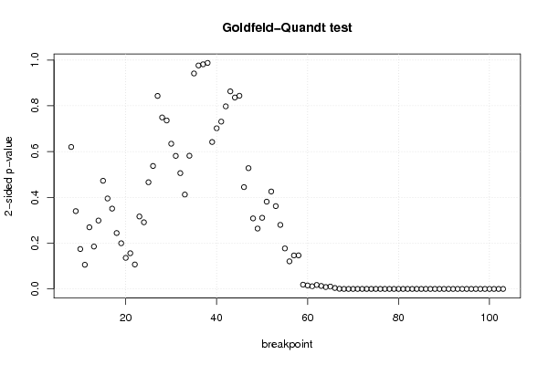
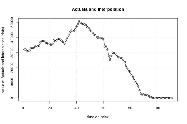
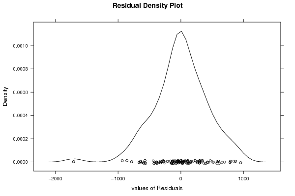
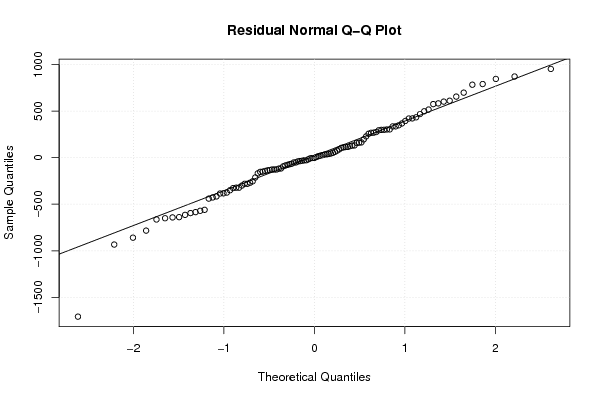
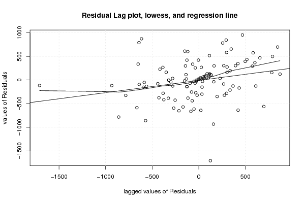
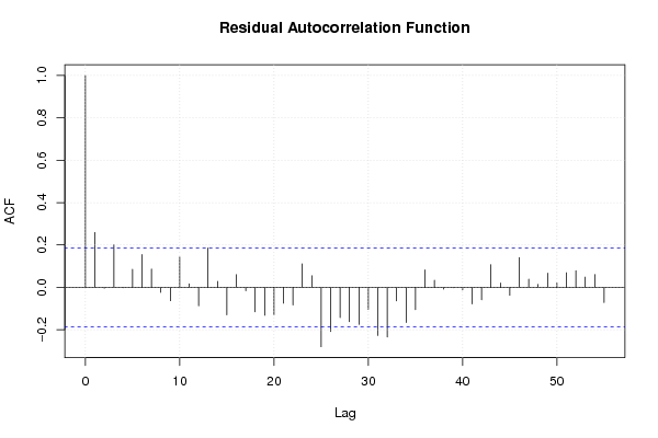
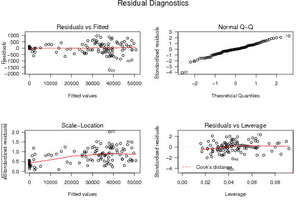
library(lattice) library(lmtest) n25 <- 25 #minimum number of obs. for Goldfeld-Quandt test par1 <- as.numeric(par1) x <- t(y) k <- length(x[1,]) n <- length(x[,1]) x1 <- cbind(x[,par1], x[,1:k!=par1]) mycolnames <- c(colnames(x)[par1], colnames(x)[1:k!=par1]) colnames(x1) <- mycolnames #colnames(x)[par1] x <- x1 if (par3 == 'First Differences'){ x2 <- array(0, dim=c(n-1,k), dimnames=list(1:(n-1), paste('(1-B)',colnames(x),sep=''))) for (i in 1:n-1) { for (j in 1:k) { x2[i,j] <- x[i+1,j] - x[i,j] } } x <- x2 } if (par2 == 'Include Monthly Dummies'){ x2 <- array(0, dim=c(n,11), dimnames=list(1:n, paste('M', seq(1:11), sep =''))) for (i in 1:11){ x2[seq(i,n,12),i] <- 1 } x <- cbind(x, x2) } if (par2 == 'Include Quarterly Dummies'){ x2 <- array(0, dim=c(n,3), dimnames=list(1:n, paste('Q', seq(1:3), sep =''))) for (i in 1:3){ x2[seq(i,n,4),i] <- 1 } x <- cbind(x, x2) } k <- length(x[1,]) if (par3 == 'Linear Trend'){ x <- cbind(x, c(1:n)) colnames(x)[k+1] <- 't' } x k <- length(x[1,]) df <- as.data.frame(x) (mylm <- lm(df)) (mysum <- summary(mylm)) if (n > n25) { kp3 <- k + 3 nmkm3 <- n - k - 3 gqarr <- array(NA, dim=c(nmkm3-kp3+1,3)) numgqtests <- 0 numsignificant1 <- 0 numsignificant5 <- 0 numsignificant10 <- 0 for (mypoint in kp3:nmkm3) { j <- 0 numgqtests <- numgqtests + 1 for (myalt in c('greater', 'two.sided', 'less')) { j <- j + 1 gqarr[mypoint-kp3+1,j] <- gqtest(mylm, point=mypoint, alternative=myalt)$p.value } if (gqarr[mypoint-kp3+1,2] < 0.01) numsignificant1 <- numsignificant1 + 1 if (gqarr[mypoint-kp3+1,2] < 0.05) numsignificant5 <- numsignificant5 + 1 if (gqarr[mypoint-kp3+1,2] < 0.10) numsignificant10 <- numsignificant10 + 1 } gqarr } bitmap(file='test0.png') plot(x[,1], type='l', main='Actuals and Interpolation', ylab='value of Actuals and Interpolation (dots)', xlab='time or index') points(x[,1]-mysum$resid) grid() dev.off() bitmap(file='test1.png') plot(mysum$resid, type='b', pch=19, main='Residuals', ylab='value of Residuals', xlab='time or index') grid() dev.off() bitmap(file='test2.png') hist(mysum$resid, main='Residual Histogram', xlab='values of Residuals') grid() dev.off() bitmap(file='test3.png') densityplot(~mysum$resid,col='black',main='Residual Density Plot', xlab='values of Residuals') dev.off() bitmap(file='test4.png') qqnorm(mysum$resid, main='Residual Normal Q-Q Plot') qqline(mysum$resid) grid() dev.off() (myerror <- as.ts(mysum$resid)) bitmap(file='test5.png') dum <- cbind(lag(myerror,k=1),myerror) dum dum1 <- dum[2:length(myerror),] dum1 z <- as.data.frame(dum1) z plot(z,main=paste('Residual Lag plot, lowess, and regression line'), ylab='values of Residuals', xlab='lagged values of Residuals') lines(lowess(z)) abline(lm(z)) grid() dev.off() bitmap(file='test6.png') acf(mysum$resid, lag.max=length(mysum$resid)/2, main='Residual Autocorrelation Function') grid() dev.off() bitmap(file='test7.png') pacf(mysum$resid, lag.max=length(mysum$resid)/2, main='Residual Partial Autocorrelation Function') grid() dev.off() bitmap(file='test8.png') opar <- par(mfrow = c(2,2), oma = c(0, 0, 1.1, 0)) plot(mylm, las = 1, sub='Residual Diagnostics') par(opar) dev.off() if (n > n25) { bitmap(file='test9.png') plot(kp3:nmkm3,gqarr[,2], main='Goldfeld-Quandt test',ylab='2-sided p-value',xlab='breakpoint') grid() dev.off() } load(file='createtable') a<-table.start() a<-table.row.start(a) a<-table.element(a, 'Multiple Linear Regression - Estimated Regression Equation', 1, TRUE) a<-table.row.end(a) myeq <- colnames(x)[1] myeq <- paste(myeq, '[t] = ', sep='') for (i in 1:k){ if (mysum$coefficients[i,1] > 0) myeq <- paste(myeq, '+', '') myeq <- paste(myeq, mysum$coefficients[i,1], sep=' ') if (rownames(mysum$coefficients)[i] != '(Intercept)') { myeq <- paste(myeq, rownames(mysum$coefficients)[i], sep='') if (rownames(mysum$coefficients)[i] != 't') myeq <- paste(myeq, '[t]', sep='') } } myeq <- paste(myeq, ' + e[t]') a<-table.row.start(a) a<-table.element(a, myeq) a<-table.row.end(a) a<-table.end(a) table.save(a,file='mytable1.tab') a<-table.start() a<-table.row.start(a) a<-table.element(a,hyperlink('http://www.xycoon.com/ols1.htm','Multiple Linear Regression - Ordinary Least Squares',''), 6, TRUE) a<-table.row.end(a) a<-table.row.start(a) a<-table.element(a,'Variable',header=TRUE) a<-table.element(a,'Parameter',header=TRUE) a<-table.element(a,'S.D.',header=TRUE) a<-table.element(a,'T-STAT<br />H0: parameter = 0',header=TRUE) a<-table.element(a,'2-tail p-value',header=TRUE) a<-table.element(a,'1-tail p-value',header=TRUE) a<-table.row.end(a) for (i in 1:k){ a<-table.row.start(a) a<-table.element(a,rownames(mysum$coefficients)[i],header=TRUE) a<-table.element(a,mysum$coefficients[i,1]) a<-table.element(a, round(mysum$coefficients[i,2],6)) a<-table.element(a, round(mysum$coefficients[i,3],4)) a<-table.element(a, round(mysum$coefficients[i,4],6)) a<-table.element(a, round(mysum$coefficients[i,4]/2,6)) a<-table.row.end(a) } a<-table.end(a) table.save(a,file='mytable2.tab') a<-table.start() a<-table.row.start(a) a<-table.element(a, 'Multiple Linear Regression - Regression Statistics', 2, TRUE) a<-table.row.end(a) a<-table.row.start(a) a<-table.element(a, 'Multiple R',1,TRUE) a<-table.element(a, sqrt(mysum$r.squared)) a<-table.row.end(a) a<-table.row.start(a) a<-table.element(a, 'R-squared',1,TRUE) a<-table.element(a, mysum$r.squared) a<-table.row.end(a) a<-table.row.start(a) a<-table.element(a, 'Adjusted R-squared',1,TRUE) a<-table.element(a, mysum$adj.r.squared) a<-table.row.end(a) a<-table.row.start(a) a<-table.element(a, 'F-TEST (value)',1,TRUE) a<-table.element(a, mysum$fstatistic[1]) a<-table.row.end(a) a<-table.row.start(a) a<-table.element(a, 'F-TEST (DF numerator)',1,TRUE) a<-table.element(a, mysum$fstatistic[2]) a<-table.row.end(a) a<-table.row.start(a) a<-table.element(a, 'F-TEST (DF denominator)',1,TRUE) a<-table.element(a, mysum$fstatistic[3]) a<-table.row.end(a) a<-table.row.start(a) a<-table.element(a, 'p-value',1,TRUE) a<-table.element(a, 1-pf(mysum$fstatistic[1],mysum$fstatistic[2],mysum$fstatistic[3])) a<-table.row.end(a) a<-table.row.start(a) a<-table.element(a, 'Multiple Linear Regression - Residual Statistics', 2, TRUE) a<-table.row.end(a) a<-table.row.start(a) a<-table.element(a, 'Residual Standard Deviation',1,TRUE) a<-table.element(a, mysum$sigma) a<-table.row.end(a) a<-table.row.start(a) a<-table.element(a, 'Sum Squared Residuals',1,TRUE) a<-table.element(a, sum(myerror*myerror)) a<-table.row.end(a) a<-table.end(a) table.save(a,file='mytable3.tab') a<-table.start() a<-table.row.start(a) a<-table.element(a, 'Multiple Linear Regression - Actuals, Interpolation, and Residuals', 4, TRUE) a<-table.row.end(a) a<-table.row.start(a) a<-table.element(a, 'Time or Index', 1, TRUE) a<-table.element(a, 'Actuals', 1, TRUE) a<-table.element(a, 'Interpolation<br />Forecast', 1, TRUE) a<-table.element(a, 'Residuals<br />Prediction Error', 1, TRUE) a<-table.row.end(a) for (i in 1:n) { a<-table.row.start(a) a<-table.element(a,i, 1, TRUE) a<-table.element(a,x[i]) a<-table.element(a,x[i]-mysum$resid[i]) a<-table.element(a,mysum$resid[i]) a<-table.row.end(a) } a<-table.end(a) table.save(a,file='mytable4.tab') if (n > n25) { a<-table.start() a<-table.row.start(a) a<-table.element(a,'Goldfeld-Quandt test for Heteroskedasticity',4,TRUE) a<-table.row.end(a) a<-table.row.start(a) a<-table.element(a,'p-values',header=TRUE) a<-table.element(a,'Alternative Hypothesis',3,header=TRUE) a<-table.row.end(a) a<-table.row.start(a) a<-table.element(a,'breakpoint index',header=TRUE) a<-table.element(a,'greater',header=TRUE) a<-table.element(a,'2-sided',header=TRUE) a<-table.element(a,'less',header=TRUE) a<-table.row.end(a) for (mypoint in kp3:nmkm3) { a<-table.row.start(a) a<-table.element(a,mypoint,header=TRUE) a<-table.element(a,gqarr[mypoint-kp3+1,1]) a<-table.element(a,gqarr[mypoint-kp3+1,2]) a<-table.element(a,gqarr[mypoint-kp3+1,3]) a<-table.row.end(a) } a<-table.end(a) table.save(a,file='mytable5.tab') a<-table.start() a<-table.row.start(a) a<-table.element(a,'Meta Analysis of Goldfeld-Quandt test for Heteroskedasticity',4,TRUE) a<-table.row.end(a) a<-table.row.start(a) a<-table.element(a,'Description',header=TRUE) a<-table.element(a,'# significant tests',header=TRUE) a<-table.element(a,'% significant tests',header=TRUE) a<-table.element(a,'OK/NOK',header=TRUE) a<-table.row.end(a) a<-table.row.start(a) a<-table.element(a,'1% type I error level',header=TRUE) a<-table.element(a,numsignificant1) a<-table.element(a,numsignificant1/numgqtests) if (numsignificant1/numgqtests < 0.01) dum <- 'OK' else dum <- 'NOK' a<-table.element(a,dum) a<-table.row.end(a) a<-table.row.start(a) a<-table.element(a,'5% type I error level',header=TRUE) a<-table.element(a,numsignificant5) a<-table.element(a,numsignificant5/numgqtests) if (numsignificant5/numgqtests < 0.05) dum <- 'OK' else dum <- 'NOK' a<-table.element(a,dum) a<-table.row.end(a) a<-table.row.start(a) a<-table.element(a,'10% type I error level',header=TRUE) a<-table.element(a,numsignificant10) a<-table.element(a,numsignificant10/numgqtests) if (numsignificant10/numgqtests < 0.1) dum <- 'OK' else dum <- 'NOK' a<-table.element(a,dum) a<-table.row.end(a) a<-table.end(a) table.save(a,file='mytable6.tab') }

Copyright

This work is licensed under a Creative Commons Attribution-Noncommercial-Share Alike 3.0 License.

Software written by Ed van Stee & Patrick Wessa

Disclaimer

Information provided on this web site is provided "AS IS" without warranty of any kind, either express or implied, including, without limitation, warranties of merchantability, fitness for a particular purpose, and noninfringement. We use reasonable efforts to include accurate and timely information and periodically update the information, and software without notice. However, we make no warranties or representations as to the accuracy or completeness of such information (or software), and we assume no liability or responsibility for errors or omissions in the content of this web site, or any software bugs in online applications. Your use of this web site is AT YOUR OWN RISK. Under no circumstances and under no legal theory shall we be liable to you or any other person for any direct, indirect, special, incidental, exemplary, or consequential damages arising from your access to, or use of, this web site.

Privacy Policy

We may request personal information to be submitted to our servers in order to be able to:

• personalize online software applications according to your needs
• enforce strict security rules with respect to the data that you upload (e.g. statistical data)
• manage user sessions of online applications
• alert you about important changes or upgrades in resources or applications

We NEVER allow other companies to directly offer registered users information about their products and services. Banner references and hyperlinks of third parties NEVER contain any personal data of the visitor.

We do NOT sell, nor transmit by any means, personal information, nor statistical data series uploaded by you to third parties.

We carefully protect your data from loss, misuse, alteration, and destruction. However, at any time, and under any circumstance you are solely responsible for managing your passwords, and keeping them secret.

We store a unique ANONYMOUS USER ID in the form of a small 'Cookie' on your computer. This allows us to track your progress when using this website which is necessary to create state-dependent features. The cookie is used for NO OTHER PURPOSE. At any time you may opt to disallow cookies from this website - this will not affect other features of this website.

We examine cookies that are used by third-parties (banner and online ads) very closely: abuse from third-parties automatically results in termination of the advertising contract without refund. We have very good reason to believe that the cookies that are produced by third parties (banner ads) do NOT cause any privacy or security risk.

FreeStatistics.org is safe. There is no need to download any software to use the applications and services contained in this website. Hence, your system's security is not compromised by their use, and your personal data - other than data you submit in the account application form, and the user-agent information that is transmitted by your browser - is never transmitted to our servers.

As a general rule, we do not log on-line behavior of individuals (other than normal logging of webserver 'hits'). However, in cases of abuse, hacking, unauthorized access, Denial of Service attacks, illegal copying, hotlinking, non-compliance with international webstandards (such as robots.txt), or any other harmful behavior, our system engineers are empowered to log, track, identify, publish, and ban misbehaving individuals - even if this leads to ban entire blocks of IP addresses, or disclosing user's identity.

FreeStatistics.org is powered by