Free Statistics
of Irreproducible Research!
Description of Statistical Computation | |||||||||||||||||||||
|---|---|---|---|---|---|---|---|---|---|---|---|---|---|---|---|---|---|---|---|---|---|
| Author's title | |||||||||||||||||||||
| Author | *The author of this computation has been verified* | ||||||||||||||||||||
| R Software Module | rwasp_meanplot.wasp | ||||||||||||||||||||
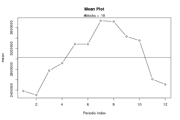
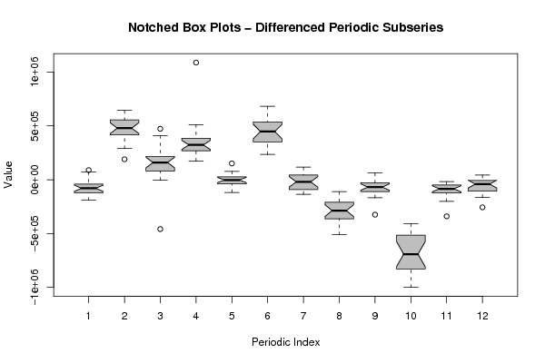
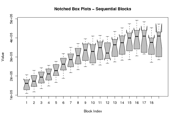
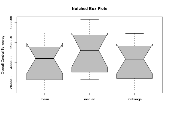
| Title produced by software | Mean Plot | ||||||||||||||||||||
| Date of computation | Fri, 10 Dec 2010 12:51:13 +0000 | ||||||||||||||||||||
| Cite this page as follows | Statistical Computations at FreeStatistics.org, Office for Research Development and Education, URL https://freestatistics.org/blog/index.php?v=date/2010/Dec/10/t12919853860xg15h3eedl46xa.htm/, Retrieved Tue, 02 Jun 2026 07:28:00 +0000 | ||||||||||||||||||||
| Statistical Computations at FreeStatistics.org, Office for Research Development and Education, URL https://freestatistics.org/blog/index.php?pk=107617, Retrieved Tue, 02 Jun 2026 07:28:00 +0000 | |||||||||||||||||||||
| QR Codes: | |||||||||||||||||||||
|
| |||||||||||||||||||||
| Original text written by user: | |||||||||||||||||||||
| IsPrivate? | No (this computation is public) | ||||||||||||||||||||
| User-defined keywords | |||||||||||||||||||||
| Estimated Impact | 519 | ||||||||||||||||||||
Tree of Dependent Computations | |||||||||||||||||||||
| Family? (F = Feedback message, R = changed R code, M = changed R Module, P = changed Parameters, D = changed Data) | |||||||||||||||||||||
| - [Linear Regression Graphical Model Validation] [Colombia Coffee -...] [2008-02-26 10:22:06] [74be16979710d4c4e7c6647856088456] - RM D [Linear Regression Graphical Model Validation] [Regressiemodel 1] [2010-11-06 16:54:19] [97ad38b1c3b35a5feca8b85f7bc7b3ff] - RMPD [Mean Plot] [Mean plot Schiphol] [2010-12-10 12:51:13] [9ea95e194e0eb2a674315798620d5bc6] [Current] | |||||||||||||||||||||
| Feedback Forum | |||||||||||||||||||||
Post a new message | |||||||||||||||||||||
Dataset | |||||||||||||||||||||
| Dataseries X: | |||||||||||||||||||||
1149822 1086979 1276674 1522522 1742117 1737275 1979900 2061036 1867943 1707752 1298756 1281814 1281151 1164976 1454329 1645288 1817743 1895785 2236311 2295951 2087315 1980891 1465446 1445026 1488120 1338333 1715789 1806090 2083316 2092278 2430800 2424894 2299016 2130688 1652221 1608162 1647074 1479691 1884978 2007898 2208954 2217164 2534291 2560312 2429069 2315077 1799608 1772590 1744799 1659093 2099821 2135736 2427894 2468882 2703217 2766841 2655236 2550373 2052097 1998055 1920748 1876694 2380930 2467402 2770771 2781340 3143926 3172235 2952540 2920877 2384552 2248987 2208616 2178756 2632870 2706905 3029745 3015402 3391414 3507805 3177852 3142961 2545815 2414007 2372578 2332664 2825328 2901478 3263955 3226738 3610786 3709274 3467185 3449646 2802951 2462530 2490645 2561520 3067554 3226951 3546493 3492787 3952263 3932072 3720284 3651555 2914972 2713514 2703997 2591373 3163748 3355137 3613702 3686773 4098716 4063517 3551489 3226663 2656842 2597484 2572399 2596631 3165225 3303145 3698247 3668631 4130433 4131400 3864358 3721110 2892532 2843451 2747502 2668775 3018602 3013392 3393657 3544233 4075832 4032923 3734509 3761285 2970090 2847849 2741680 2830639 3257673 3480085 3843271 3796961 4337767 4243630 3927202 3915296 3087396 2963792 2955792 2829925 3281195 3548011 4059648 3941175 4528594 4433151 4145737 4077132 3198519 3078660 3028202 2858642 3398954 3808883 4175961 4227542 4744616 4608012 4295049 4201144 3353276 3286851 3169889 3051720 3695426 3905501 4296458 4246247 4921849 4821446 4425064 4379099 3472889 3359160 3200944 3153170 3741498 3918719 4403449 4400407 4847473 4716136 4297440 4272253 3271834 3168388 2911748 2720999 3199918 3672623 3892013 3850845 4532467 4484739 4014972 3983758 3158459 3100569 2935404 2855719 3465611 3006985 4095110 4104793 4730788 4642726 4246919 4308117 | |||||||||||||||||||||
Tables (Output of Computation) | |||||||||||||||||||||
| |||||||||||||||||||||
Figures (Output of Computation) | |||||||||||||||||||||
Input Parameters & R Code | |||||||||||||||||||||
| Parameters (Session): | |||||||||||||||||||||
| par1 = 12 ; | |||||||||||||||||||||
| Parameters (R input): | |||||||||||||||||||||
| par1 = 12 ; | |||||||||||||||||||||
| R code (references can be found in the software module): | |||||||||||||||||||||
par1 <- as.numeric(par1) | |||||||||||||||||||||