Free Statistics
of Irreproducible Research!
Description of Statistical Computation | |||||||||||||||||||||||||||||||||||||||||||||||||||||||||||||
|---|---|---|---|---|---|---|---|---|---|---|---|---|---|---|---|---|---|---|---|---|---|---|---|---|---|---|---|---|---|---|---|---|---|---|---|---|---|---|---|---|---|---|---|---|---|---|---|---|---|---|---|---|---|---|---|---|---|---|---|---|---|
| Author's title | |||||||||||||||||||||||||||||||||||||||||||||||||||||||||||||
| Author | *The author of this computation has been verified* | ||||||||||||||||||||||||||||||||||||||||||||||||||||||||||||
| R Software Module | rwasp_linear_regression.wasp | ||||||||||||||||||||||||||||||||||||||||||||||||||||||||||||
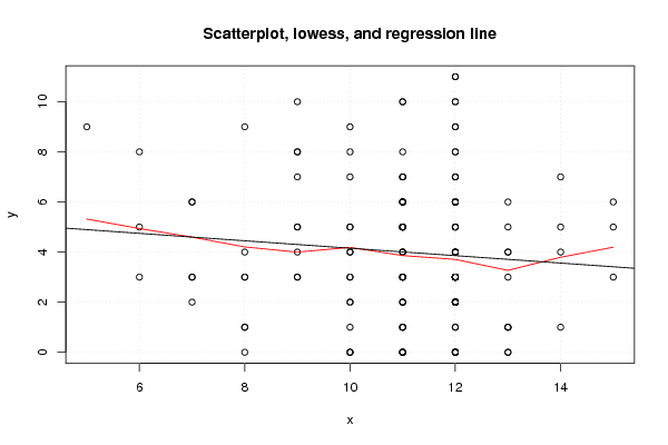
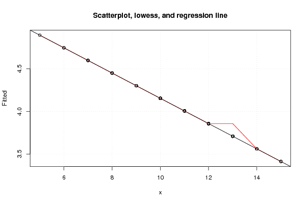
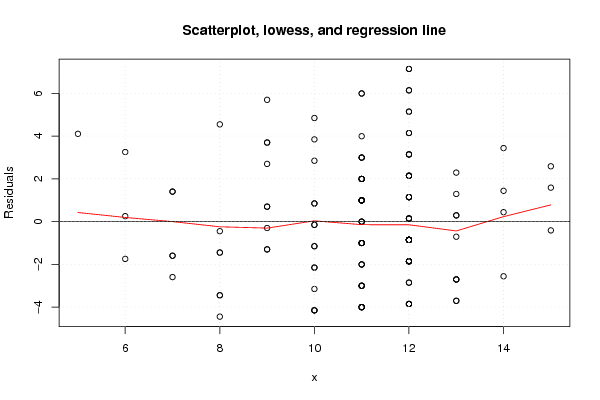
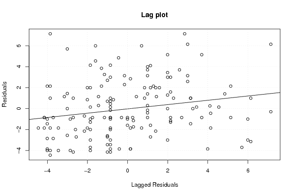
| Title produced by software | Linear Regression Graphical Model Validation | ||||||||||||||||||||||||||||||||||||||||||||||||||||||||||||
| Date of computation | Thu, 09 Dec 2010 19:40:21 +0000 | ||||||||||||||||||||||||||||||||||||||||||||||||||||||||||||
| Cite this page as follows | Statistical Computations at FreeStatistics.org, Office for Research Development and Education, URL https://freestatistics.org/blog/index.php?v=date/2010/Dec/09/t1291923518u0v0d8c4lpdolvi.htm/, Retrieved Sat, 10 Jan 2026 08:33:39 +0000 | ||||||||||||||||||||||||||||||||||||||||||||||||||||||||||||
| Statistical Computations at FreeStatistics.org, Office for Research Development and Education, URL https://freestatistics.org/blog/index.php?pk=107366, Retrieved Sat, 10 Jan 2026 08:33:39 +0000 | |||||||||||||||||||||||||||||||||||||||||||||||||||||||||||||
| QR Codes: | |||||||||||||||||||||||||||||||||||||||||||||||||||||||||||||
|
| |||||||||||||||||||||||||||||||||||||||||||||||||||||||||||||
| Original text written by user: | |||||||||||||||||||||||||||||||||||||||||||||||||||||||||||||
| IsPrivate? | No (this computation is public) | ||||||||||||||||||||||||||||||||||||||||||||||||||||||||||||
| User-defined keywords | |||||||||||||||||||||||||||||||||||||||||||||||||||||||||||||
| Estimated Impact | 424 | ||||||||||||||||||||||||||||||||||||||||||||||||||||||||||||
Tree of Dependent Computations | |||||||||||||||||||||||||||||||||||||||||||||||||||||||||||||
| Family? (F = Feedback message, R = changed R code, M = changed R Module, P = changed Parameters, D = changed Data) | |||||||||||||||||||||||||||||||||||||||||||||||||||||||||||||
| - [Linear Regression Graphical Model Validation] [Colombia Coffee -...] [2008-02-26 10:22:06] [74be16979710d4c4e7c6647856088456] - M D [Linear Regression Graphical Model Validation] [workshop 6 tutorial] [2010-11-12 10:13:29] [87d60b8864dc39f7ed759c345edfb471] - D [Linear Regression Graphical Model Validation] [workshop 6 mini-t...] [2010-11-12 14:05:27] [87d60b8864dc39f7ed759c345edfb471] - D [Linear Regression Graphical Model Validation] [W6-mini tutorial] [2010-11-12 20:07:18] [48146708a479232c43a8f6e52fbf83b4] - D [Linear Regression Graphical Model Validation] [tutorial 1] [2010-11-17 02:46:03] [c61422349906618fd7554832db11aa8e] - D [Linear Regression Graphical Model Validation] [tutorial 2] [2010-11-17 03:21:42] [c61422349906618fd7554832db11aa8e] - D [Linear Regression Graphical Model Validation] [Simple Linear Reg...] [2010-12-09 19:40:21] [1638ccfec791c539017705f3e680eb33] [Current] | |||||||||||||||||||||||||||||||||||||||||||||||||||||||||||||
| Feedback Forum | |||||||||||||||||||||||||||||||||||||||||||||||||||||||||||||
Post a new message | |||||||||||||||||||||||||||||||||||||||||||||||||||||||||||||
Dataset | |||||||||||||||||||||||||||||||||||||||||||||||||||||||||||||
| Dataseries X: | |||||||||||||||||||||||||||||||||||||||||||||||||||||||||||||
10 9 12 12 9 11 12 11 12 12 11 11 12 6 13 11 12 10 11 12 12 12 11 12 12 12 6 5 12 14 12 9 11 11 11 12 10 12 11 12 9 15 11 11 15 12 9 12 9 11 12 11 6 10 12 13 11 10 11 7 11 11 7 12 14 11 12 11 12 12 12 12 15 11 13 10 12 13 14 11 11 7 11 12 12 10 12 8 7 11 11 11 9 12 13 9 11 12 9 12 12 12 14 11 12 8 12 12 12 11 11 12 10 13 8 12 11 10 13 10 10 7 10 8 12 12 12 11 13 12 8 11 12 13 12 10 12 10 13 11 12 12 10 11 11 11 8 11 12 11 12 12 12 8 12 11 | |||||||||||||||||||||||||||||||||||||||||||||||||||||||||||||
| Dataseries Y: | |||||||||||||||||||||||||||||||||||||||||||||||||||||||||||||
8 3 6 9 8 5 7 7 6 0 8 5 3 3 4 5 7 4 5 0 3 6 0 2 4 3 5 9 5 4 3 7 3 4 6 5 1 10 7 3 8 6 7 6 5 6 3 2 5 3 3 4 8 3 6 5 6 5 2 2 3 10 3 5 5 1 2 2 2 8 2 0 3 5 6 4 3 1 1 1 6 6 5 10 11 7 4 9 3 4 1 10 5 3 0 10 1 3 4 11 0 4 7 6 2 1 3 3 9 6 2 3 3 4 3 7 5 5 3 2 2 6 9 4 8 3 3 5 1 5 3 0 1 0 2 0 3 0 1 3 2 3 0 3 0 0 1 3 1 0 0 4 2 0 0 0 | |||||||||||||||||||||||||||||||||||||||||||||||||||||||||||||
Tables (Output of Computation) | |||||||||||||||||||||||||||||||||||||||||||||||||||||||||||||
| |||||||||||||||||||||||||||||||||||||||||||||||||||||||||||||
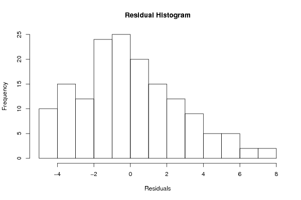
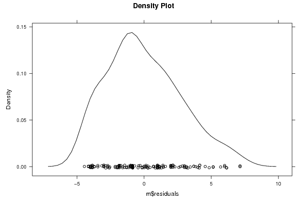
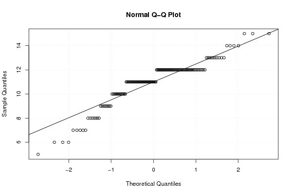
Figures (Output of Computation) | |||||||||||||||||||||||||||||||||||||||||||||||||||||||||||||
Input Parameters & R Code | |||||||||||||||||||||||||||||||||||||||||||||||||||||||||||||
| Parameters (Session): | |||||||||||||||||||||||||||||||||||||||||||||||||||||||||||||
| par1 = 0 ; | |||||||||||||||||||||||||||||||||||||||||||||||||||||||||||||
| Parameters (R input): | |||||||||||||||||||||||||||||||||||||||||||||||||||||||||||||
| par1 = 0 ; | |||||||||||||||||||||||||||||||||||||||||||||||||||||||||||||
| R code (references can be found in the software module): | |||||||||||||||||||||||||||||||||||||||||||||||||||||||||||||
par1 <- as.numeric(par1) | |||||||||||||||||||||||||||||||||||||||||||||||||||||||||||||