Free Statistics
of Irreproducible Research!
Description of Statistical Computation | |||||||||||||||||||||||||||||||||||||||||||||||||||||
|---|---|---|---|---|---|---|---|---|---|---|---|---|---|---|---|---|---|---|---|---|---|---|---|---|---|---|---|---|---|---|---|---|---|---|---|---|---|---|---|---|---|---|---|---|---|---|---|---|---|---|---|---|---|
| Author's title | |||||||||||||||||||||||||||||||||||||||||||||||||||||
| Author | *The author of this computation has been verified* | ||||||||||||||||||||||||||||||||||||||||||||||||||||
| R Software Module | rwasp_edauni.wasp | ||||||||||||||||||||||||||||||||||||||||||||||||||||
| Title produced by software | Univariate Explorative Data Analysis | ||||||||||||||||||||||||||||||||||||||||||||||||||||
| Date of computation | Sat, 04 Dec 2010 10:09:17 +0000 | ||||||||||||||||||||||||||||||||||||||||||||||||||||
| Cite this page as follows | Statistical Computations at FreeStatistics.org, Office for Research Development and Education, URL https://freestatistics.org/blog/index.php?v=date/2010/Dec/04/t12914572607dbb4v4m5xhqqkr.htm/, Retrieved Thu, 28 May 2026 07:44:12 +0000 | ||||||||||||||||||||||||||||||||||||||||||||||||||||
| Statistical Computations at FreeStatistics.org, Office for Research Development and Education, URL https://freestatistics.org/blog/index.php?pk=105068, Retrieved Thu, 28 May 2026 07:44:12 +0000 | |||||||||||||||||||||||||||||||||||||||||||||||||||||
| QR Codes: | |||||||||||||||||||||||||||||||||||||||||||||||||||||
|
| |||||||||||||||||||||||||||||||||||||||||||||||||||||
| Original text written by user: | |||||||||||||||||||||||||||||||||||||||||||||||||||||
| IsPrivate? | No (this computation is public) | ||||||||||||||||||||||||||||||||||||||||||||||||||||
| User-defined keywords | |||||||||||||||||||||||||||||||||||||||||||||||||||||
| Estimated Impact | 491 | ||||||||||||||||||||||||||||||||||||||||||||||||||||
Tree of Dependent Computations | |||||||||||||||||||||||||||||||||||||||||||||||||||||
| Family? (F = Feedback message, R = changed R code, M = changed R Module, P = changed Parameters, D = changed Data) | |||||||||||||||||||||||||||||||||||||||||||||||||||||
| - [Central Tendency] [SHW_WS3_Yt=c+Xt] [2009-10-16 08:10:06] [8b1aef4e7013bd33fbc2a5833375c5f5] - RMPD [Univariate Explorative Data Analysis] [] [2009-11-02 10:43:25] [8b1aef4e7013bd33fbc2a5833375c5f5] - PD [Univariate Explorative Data Analysis] [Paper univariate 2] [2010-12-04 10:09:17] [da925928e5a77063c5ecc7b801d712e1] [Current] - R D [Univariate Explorative Data Analysis] [] [2011-12-01 18:21:13] [74be16979710d4c4e7c6647856088456] | |||||||||||||||||||||||||||||||||||||||||||||||||||||
| Feedback Forum | |||||||||||||||||||||||||||||||||||||||||||||||||||||
Post a new message | |||||||||||||||||||||||||||||||||||||||||||||||||||||
Dataset | |||||||||||||||||||||||||||||||||||||||||||||||||||||
| Dataseries X: | |||||||||||||||||||||||||||||||||||||||||||||||||||||
-2,250815803 -2,250025575 -2,248469388 -2,249602446 -2,248990826 -2,24598369 -2,245779817 -2,245380711 -2,243004552 -2,245 -2,244359233 -2,247455919 -2,248922457 -2,248721805 -2,24955 -2,246140089 -2,244470821 -2,245559389 -2,246977887 -2,246879607 -2,248921569 -2,248486036 -2,249574156 -2,249339853 -2,245839844 -2,247176987 -2,247019932 -2,251234867 -2,253571774 -2,255750845 -2,253840231 -2,253942308 -2,253956835 -2,253815916 -2,254736842 -2,253448111 -2,254229852 -2,251706387 -2,251615055 -2,252952381 -2,255066414 -2,252336802 -2,252961738 -2,251556604 -2,251517436 -2,252561205 -2,251263504 -2,251846298 -2,252559663 -2,25411215 -2,254727018 -2,251061453 -2,247860465 -2,249532191 -2,248863216 -2,249580452 -2,250653775 -2,246850575 -2,248297384 -2,24959193 -2,249661482 -2,248259479 -2,246000912 -2,247477314 -2,248637392 -2,247013575 -2,245843102 -2,245990991 -2,245778578 -2,248898876 -2,248470166 -2,247046168 | |||||||||||||||||||||||||||||||||||||||||||||||||||||
Tables (Output of Computation) | |||||||||||||||||||||||||||||||||||||||||||||||||||||
| |||||||||||||||||||||||||||||||||||||||||||||||||||||
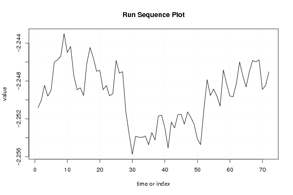
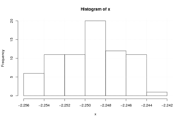
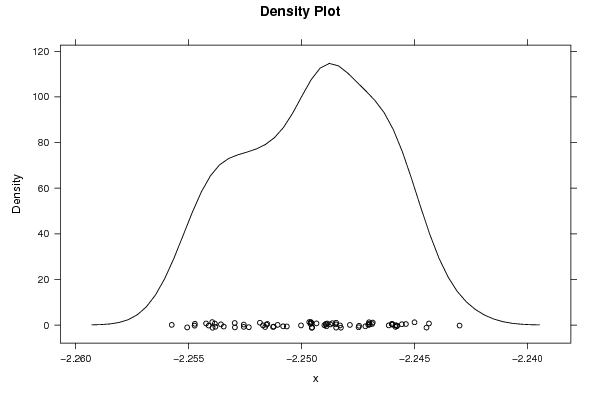
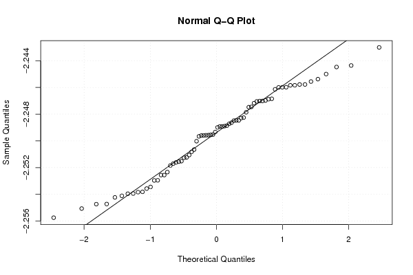
Figures (Output of Computation) | |||||||||||||||||||||||||||||||||||||||||||||||||||||
Input Parameters & R Code | |||||||||||||||||||||||||||||||||||||||||||||||||||||
| Parameters (Session): | |||||||||||||||||||||||||||||||||||||||||||||||||||||
| par1 = 0 ; par2 = 0 ; | |||||||||||||||||||||||||||||||||||||||||||||||||||||
| Parameters (R input): | |||||||||||||||||||||||||||||||||||||||||||||||||||||
| par1 = 0 ; par2 = 0 ; | |||||||||||||||||||||||||||||||||||||||||||||||||||||
| R code (references can be found in the software module): | |||||||||||||||||||||||||||||||||||||||||||||||||||||
par1 <- as.numeric(par1) | |||||||||||||||||||||||||||||||||||||||||||||||||||||