Repository of Reproducible Computations

Free Statistics

of Irreproducible Research!

Author's title

Author

*The author of this computation has been verified*

R Software Module

rwasp_autocorrelation.wasp

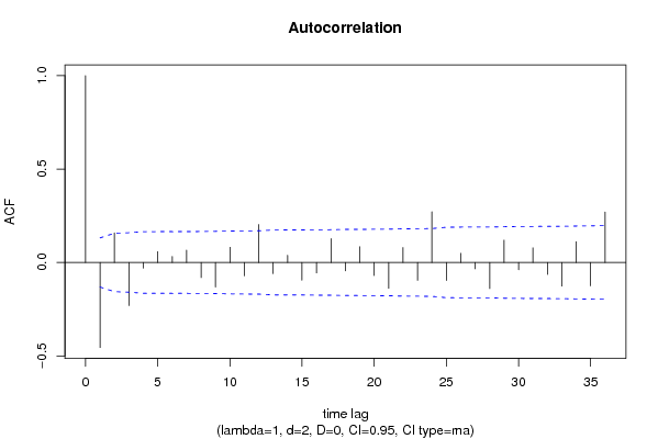
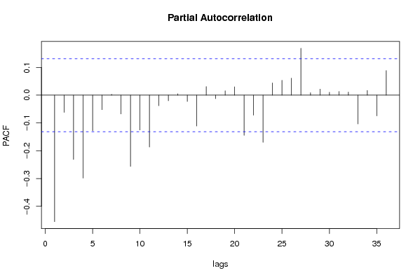
Title produced by software

(Partial) Autocorrelation Function

Date of computation

Mon, 30 Nov 2009 13:25:55 -0700

Cite this page as follows

Statistical Computations at FreeStatistics.org, Office for Research Development and Education, URL https://freestatistics.org/blog/index.php?v=date/2009/Nov/30/t1259612793lmisc8lhrnnv89o.htm/, Retrieved Mon, 29 Apr 2024 01:56:32 +0000

Statistical Computations at FreeStatistics.org, Office for Research Development and Education, URL https://freestatistics.org/blog/index.php?pk=61887, Retrieved Mon, 29 Apr 2024 01:56:32 +0000

QR Codes:

Paste this QR Code to cite your computation.

Original text written by user:

IsPrivate?

No (this computation is public)

User-defined keywords

Estimated Impact

158

Family? (F = Feedback message, R = changed R code, M = changed R Module, P = changed Parameters, D = changed Data)

-     [Univariate Explorative Data Analysis] [Run Sequence gebo...] [2008-12-12 13:32:37] [76963dc1903f0f612b6153510a3818cf]
- R  D  [Univariate Explorative Data Analysis] [Run Sequence gebo...] [2008-12-17 12:14:40] [76963dc1903f0f612b6153510a3818cf]
-         [Univariate Explorative Data Analysis] [Run Sequence Plot...] [2008-12-22 18:19:51] [1ce0d16c8f4225c977b42c8fa93bc163]
- RMP       [(Partial) Autocorrelation Function] [Identifying Integ...] [2009-11-22 12:16:10] [b98453cac15ba1066b407e146608df68]
-   PD        [(Partial) Autocorrelation Function] [ws8_2] [2009-11-24 20:22:15] [8b1aef4e7013bd33fbc2a5833375c5f5]
-   P           [(Partial) Autocorrelation Function] [WS8_seizonaliteit1] [2009-11-25 17:44:58] [8b1aef4e7013bd33fbc2a5833375c5f5]
-                   [(Partial) Autocorrelation Function] [review WS 8 autoc...] [2009-11-30 20:25:55] [51d49d3536f6a59f2486a67bf50b2759] [Current]

Feedback Forum

Post a new message

Dataseries X:

Download CSV

Histogram

Boxplots

Summary of computational transaction
Raw Input	view raw input (R code)
Raw Output	view raw output of R engine
Computing time	1 seconds
R Server	'Gwilym Jenkins' @ 72.249.127.135

\begin{tabular}{lllllllll}
\hline
Summary of computational transaction \tabularnewline
Raw Input & view raw input (R code)  \tabularnewline
Raw Output & view raw output of R engine  \tabularnewline
Computing time & 1 seconds \tabularnewline
R Server & 'Gwilym Jenkins' @ 72.249.127.135 \tabularnewline
\hline
\end{tabular}
%Source: https://freestatistics.org/blog/index.php?pk=61887&T=0

[TABLE]
[ROW][C]Summary of computational transaction[/C][/ROW]
[ROW][C]Raw Input[/C][C]view raw input (R code) [/C][/ROW]
[ROW][C]Raw Output[/C][C]view raw output of R engine [/C][/ROW]
[ROW][C]Computing time[/C][C]1 seconds[/C][/ROW]
[ROW][C]R Server[/C][C]'Gwilym Jenkins' @ 72.249.127.135[/C][/ROW]
[/TABLE]
Source: https://freestatistics.org/blog/index.php?pk=61887&T=0

Globally Unique Identifier (entire table): ba.freestatistics.org/blog/index.php?pk=61887&T=0

As an alternative you can also use a QR Code:

The GUIDs for individual cells are displayed in the table below:

Summary of computational transaction
Raw Input	view raw input (R code)
Raw Output	view raw output of R engine
Computing time	1 seconds
R Server	'Gwilym Jenkins' @ 72.249.127.135

Autocorrelation Function
Time lag k	ACF(k)	T-STAT	P-value
1	-0.455366	-6.7848	0
2	0.158241	2.3577	0.009628
3	-0.231035	-3.4424	0.000345
4	-0.030348	-0.4522	0.325795
5	0.057954	0.8635	0.194397
6	0.032459	0.4836	0.314565
7	0.065979	0.9831	0.163323
8	-0.08107	-1.2079	0.114184
9	-0.131748	-1.963	0.025447
10	0.081048	1.2076	0.114244
11	-0.071719	-1.0686	0.143206
12	0.203266	3.0286	0.001374
13	-0.059871	-0.8921	0.186665
14	0.038385	0.5719	0.283978
15	-0.095239	-1.419	0.078647
16	-0.055768	-0.8309	0.203455
17	0.127829	1.9046	0.029062
18	-0.045362	-0.6759	0.249913
19	0.084621	1.2608	0.104347
20	-0.070235	-1.0465	0.148239
21	-0.138129	-2.0581	0.020375
22	0.079591	1.1859	0.11847
23	-0.095905	-1.429	0.077212
24	0.271772	4.0493	3.5e-05
25	-0.096122	-1.4322	0.076748
26	0.049186	0.7329	0.232211
27	-0.034391	-0.5124	0.304435
28	-0.139856	-2.0838	0.019161
29	0.11924	1.7766	0.038499
30	-0.038833	-0.5786	0.281724
31	0.0785	1.1696	0.121703
32	-0.064088	-0.9549	0.170337
33	-0.126456	-1.8841	0.030426
34	0.111412	1.66	0.049163
35	-0.124758	-1.8589	0.032185
36	0.26989	4.0213	4e-05

\begin{tabular}{lllllllll}
\hline
Autocorrelation Function \tabularnewline
Time lag k & ACF(k) & T-STAT & P-value \tabularnewline
1 & -0.455366 & -6.7848 & 0 \tabularnewline
2 & 0.158241 & 2.3577 & 0.009628 \tabularnewline
3 & -0.231035 & -3.4424 & 0.000345 \tabularnewline
4 & -0.030348 & -0.4522 & 0.325795 \tabularnewline
5 & 0.057954 & 0.8635 & 0.194397 \tabularnewline
6 & 0.032459 & 0.4836 & 0.314565 \tabularnewline
7 & 0.065979 & 0.9831 & 0.163323 \tabularnewline
8 & -0.08107 & -1.2079 & 0.114184 \tabularnewline
9 & -0.131748 & -1.963 & 0.025447 \tabularnewline
10 & 0.081048 & 1.2076 & 0.114244 \tabularnewline
11 & -0.071719 & -1.0686 & 0.143206 \tabularnewline
12 & 0.203266 & 3.0286 & 0.001374 \tabularnewline
13 & -0.059871 & -0.8921 & 0.186665 \tabularnewline
14 & 0.038385 & 0.5719 & 0.283978 \tabularnewline
15 & -0.095239 & -1.419 & 0.078647 \tabularnewline
16 & -0.055768 & -0.8309 & 0.203455 \tabularnewline
17 & 0.127829 & 1.9046 & 0.029062 \tabularnewline
18 & -0.045362 & -0.6759 & 0.249913 \tabularnewline
19 & 0.084621 & 1.2608 & 0.104347 \tabularnewline
20 & -0.070235 & -1.0465 & 0.148239 \tabularnewline
21 & -0.138129 & -2.0581 & 0.020375 \tabularnewline
22 & 0.079591 & 1.1859 & 0.11847 \tabularnewline
23 & -0.095905 & -1.429 & 0.077212 \tabularnewline
24 & 0.271772 & 4.0493 & 3.5e-05 \tabularnewline
25 & -0.096122 & -1.4322 & 0.076748 \tabularnewline
26 & 0.049186 & 0.7329 & 0.232211 \tabularnewline
27 & -0.034391 & -0.5124 & 0.304435 \tabularnewline
28 & -0.139856 & -2.0838 & 0.019161 \tabularnewline
29 & 0.11924 & 1.7766 & 0.038499 \tabularnewline
30 & -0.038833 & -0.5786 & 0.281724 \tabularnewline
31 & 0.0785 & 1.1696 & 0.121703 \tabularnewline
32 & -0.064088 & -0.9549 & 0.170337 \tabularnewline
33 & -0.126456 & -1.8841 & 0.030426 \tabularnewline
34 & 0.111412 & 1.66 & 0.049163 \tabularnewline
35 & -0.124758 & -1.8589 & 0.032185 \tabularnewline
36 & 0.26989 & 4.0213 & 4e-05 \tabularnewline
\hline
\end{tabular}
%Source: https://freestatistics.org/blog/index.php?pk=61887&T=1

[TABLE]
[ROW][C]Autocorrelation Function[/C][/ROW]
[ROW][C]Time lag k[/C][C]ACF(k)[/C][C]T-STAT[/C][C]P-value[/C][/ROW]
[ROW][C]1[/C][C]-0.455366[/C][C]-6.7848[/C][C]0[/C][/ROW]
[ROW][C]2[/C][C]0.158241[/C][C]2.3577[/C][C]0.009628[/C][/ROW]
[ROW][C]3[/C][C]-0.231035[/C][C]-3.4424[/C][C]0.000345[/C][/ROW]
[ROW][C]4[/C][C]-0.030348[/C][C]-0.4522[/C][C]0.325795[/C][/ROW]
[ROW][C]5[/C][C]0.057954[/C][C]0.8635[/C][C]0.194397[/C][/ROW]
[ROW][C]6[/C][C]0.032459[/C][C]0.4836[/C][C]0.314565[/C][/ROW]
[ROW][C]7[/C][C]0.065979[/C][C]0.9831[/C][C]0.163323[/C][/ROW]
[ROW][C]8[/C][C]-0.08107[/C][C]-1.2079[/C][C]0.114184[/C][/ROW]
[ROW][C]9[/C][C]-0.131748[/C][C]-1.963[/C][C]0.025447[/C][/ROW]
[ROW][C]10[/C][C]0.081048[/C][C]1.2076[/C][C]0.114244[/C][/ROW]
[ROW][C]11[/C][C]-0.071719[/C][C]-1.0686[/C][C]0.143206[/C][/ROW]
[ROW][C]12[/C][C]0.203266[/C][C]3.0286[/C][C]0.001374[/C][/ROW]
[ROW][C]13[/C][C]-0.059871[/C][C]-0.8921[/C][C]0.186665[/C][/ROW]
[ROW][C]14[/C][C]0.038385[/C][C]0.5719[/C][C]0.283978[/C][/ROW]
[ROW][C]15[/C][C]-0.095239[/C][C]-1.419[/C][C]0.078647[/C][/ROW]
[ROW][C]16[/C][C]-0.055768[/C][C]-0.8309[/C][C]0.203455[/C][/ROW]
[ROW][C]17[/C][C]0.127829[/C][C]1.9046[/C][C]0.029062[/C][/ROW]
[ROW][C]18[/C][C]-0.045362[/C][C]-0.6759[/C][C]0.249913[/C][/ROW]
[ROW][C]19[/C][C]0.084621[/C][C]1.2608[/C][C]0.104347[/C][/ROW]
[ROW][C]20[/C][C]-0.070235[/C][C]-1.0465[/C][C]0.148239[/C][/ROW]
[ROW][C]21[/C][C]-0.138129[/C][C]-2.0581[/C][C]0.020375[/C][/ROW]
[ROW][C]22[/C][C]0.079591[/C][C]1.1859[/C][C]0.11847[/C][/ROW]
[ROW][C]23[/C][C]-0.095905[/C][C]-1.429[/C][C]0.077212[/C][/ROW]
[ROW][C]24[/C][C]0.271772[/C][C]4.0493[/C][C]3.5e-05[/C][/ROW]
[ROW][C]25[/C][C]-0.096122[/C][C]-1.4322[/C][C]0.076748[/C][/ROW]
[ROW][C]26[/C][C]0.049186[/C][C]0.7329[/C][C]0.232211[/C][/ROW]
[ROW][C]27[/C][C]-0.034391[/C][C]-0.5124[/C][C]0.304435[/C][/ROW]
[ROW][C]28[/C][C]-0.139856[/C][C]-2.0838[/C][C]0.019161[/C][/ROW]
[ROW][C]29[/C][C]0.11924[/C][C]1.7766[/C][C]0.038499[/C][/ROW]
[ROW][C]30[/C][C]-0.038833[/C][C]-0.5786[/C][C]0.281724[/C][/ROW]
[ROW][C]31[/C][C]0.0785[/C][C]1.1696[/C][C]0.121703[/C][/ROW]
[ROW][C]32[/C][C]-0.064088[/C][C]-0.9549[/C][C]0.170337[/C][/ROW]
[ROW][C]33[/C][C]-0.126456[/C][C]-1.8841[/C][C]0.030426[/C][/ROW]
[ROW][C]34[/C][C]0.111412[/C][C]1.66[/C][C]0.049163[/C][/ROW]
[ROW][C]35[/C][C]-0.124758[/C][C]-1.8589[/C][C]0.032185[/C][/ROW]
[ROW][C]36[/C][C]0.26989[/C][C]4.0213[/C][C]4e-05[/C][/ROW]
[/TABLE]
Source: https://freestatistics.org/blog/index.php?pk=61887&T=1

Globally Unique Identifier (entire table): ba.freestatistics.org/blog/index.php?pk=61887&T=1

As an alternative you can also use a QR Code:

The GUIDs for individual cells are displayed in the table below:

Autocorrelation Function
Time lag k	ACF(k)	T-STAT	P-value
1	-0.455366	-6.7848	0
2	0.158241	2.3577	0.009628
3	-0.231035	-3.4424	0.000345
4	-0.030348	-0.4522	0.325795
5	0.057954	0.8635	0.194397
6	0.032459	0.4836	0.314565
7	0.065979	0.9831	0.163323
8	-0.08107	-1.2079	0.114184
9	-0.131748	-1.963	0.025447
10	0.081048	1.2076	0.114244
11	-0.071719	-1.0686	0.143206
12	0.203266	3.0286	0.001374
13	-0.059871	-0.8921	0.186665
14	0.038385	0.5719	0.283978
15	-0.095239	-1.419	0.078647
16	-0.055768	-0.8309	0.203455
17	0.127829	1.9046	0.029062
18	-0.045362	-0.6759	0.249913
19	0.084621	1.2608	0.104347
20	-0.070235	-1.0465	0.148239
21	-0.138129	-2.0581	0.020375
22	0.079591	1.1859	0.11847
23	-0.095905	-1.429	0.077212
24	0.271772	4.0493	3.5e-05
25	-0.096122	-1.4322	0.076748
26	0.049186	0.7329	0.232211
27	-0.034391	-0.5124	0.304435
28	-0.139856	-2.0838	0.019161
29	0.11924	1.7766	0.038499
30	-0.038833	-0.5786	0.281724
31	0.0785	1.1696	0.121703
32	-0.064088	-0.9549	0.170337
33	-0.126456	-1.8841	0.030426
34	0.111412	1.66	0.049163
35	-0.124758	-1.8589	0.032185
36	0.26989	4.0213	4e-05

Partial Autocorrelation Function
Time lag k	PACF(k)	T-STAT	P-value
1	-0.455366	-6.7848	0
2	-0.061966	-0.9233	0.178432
3	-0.231421	-3.4481	0.000338
4	-0.298741	-4.4511	7e-06
5	-0.128274	-1.9112	0.028631
6	-0.0522	-0.7778	0.218767
7	0.003312	0.0493	0.480344
8	-0.067746	-1.0094	0.156943
9	-0.256405	-3.8203	8.7e-05
10	-0.125248	-1.8662	0.031669
11	-0.186674	-2.7814	0.002939
12	-0.038071	-0.5672	0.285562
13	-0.019981	-0.2977	0.383102
14	0.004999	0.0745	0.470346
15	-0.022689	-0.3381	0.36782
16	-0.111085	-1.6551	0.049656
17	0.031063	0.4628	0.321969
18	-0.01259	-0.1876	0.425686
19	0.01575	0.2347	0.407344
20	0.030056	0.4478	0.327359
21	-0.14454	-2.1536	0.016175
22	-0.071963	-1.0722	0.142392
23	-0.169732	-2.529	0.006067
24	0.044185	0.6583	0.255499
25	0.053553	0.7979	0.212886
26	0.061156	0.9112	0.181588
27	0.168878	2.5162	0.006284
28	0.008997	0.134	0.446744
29	0.021696	0.3233	0.373401
30	0.010525	0.1568	0.437764
31	0.0133	0.1982	0.421549
32	0.011008	0.164	0.434934
33	-0.103715	-1.5453	0.061848
34	0.017214	0.2565	0.39891
35	-0.074675	-1.1126	0.133535
36	0.088505	1.3187	0.094314

\begin{tabular}{lllllllll}
\hline
Partial Autocorrelation Function \tabularnewline
Time lag k & PACF(k) & T-STAT & P-value \tabularnewline
1 & -0.455366 & -6.7848 & 0 \tabularnewline
2 & -0.061966 & -0.9233 & 0.178432 \tabularnewline
3 & -0.231421 & -3.4481 & 0.000338 \tabularnewline
4 & -0.298741 & -4.4511 & 7e-06 \tabularnewline
5 & -0.128274 & -1.9112 & 0.028631 \tabularnewline
6 & -0.0522 & -0.7778 & 0.218767 \tabularnewline
7 & 0.003312 & 0.0493 & 0.480344 \tabularnewline
8 & -0.067746 & -1.0094 & 0.156943 \tabularnewline
9 & -0.256405 & -3.8203 & 8.7e-05 \tabularnewline
10 & -0.125248 & -1.8662 & 0.031669 \tabularnewline
11 & -0.186674 & -2.7814 & 0.002939 \tabularnewline
12 & -0.038071 & -0.5672 & 0.285562 \tabularnewline
13 & -0.019981 & -0.2977 & 0.383102 \tabularnewline
14 & 0.004999 & 0.0745 & 0.470346 \tabularnewline
15 & -0.022689 & -0.3381 & 0.36782 \tabularnewline
16 & -0.111085 & -1.6551 & 0.049656 \tabularnewline
17 & 0.031063 & 0.4628 & 0.321969 \tabularnewline
18 & -0.01259 & -0.1876 & 0.425686 \tabularnewline
19 & 0.01575 & 0.2347 & 0.407344 \tabularnewline
20 & 0.030056 & 0.4478 & 0.327359 \tabularnewline
21 & -0.14454 & -2.1536 & 0.016175 \tabularnewline
22 & -0.071963 & -1.0722 & 0.142392 \tabularnewline
23 & -0.169732 & -2.529 & 0.006067 \tabularnewline
24 & 0.044185 & 0.6583 & 0.255499 \tabularnewline
25 & 0.053553 & 0.7979 & 0.212886 \tabularnewline
26 & 0.061156 & 0.9112 & 0.181588 \tabularnewline
27 & 0.168878 & 2.5162 & 0.006284 \tabularnewline
28 & 0.008997 & 0.134 & 0.446744 \tabularnewline
29 & 0.021696 & 0.3233 & 0.373401 \tabularnewline
30 & 0.010525 & 0.1568 & 0.437764 \tabularnewline
31 & 0.0133 & 0.1982 & 0.421549 \tabularnewline
32 & 0.011008 & 0.164 & 0.434934 \tabularnewline
33 & -0.103715 & -1.5453 & 0.061848 \tabularnewline
34 & 0.017214 & 0.2565 & 0.39891 \tabularnewline
35 & -0.074675 & -1.1126 & 0.133535 \tabularnewline
36 & 0.088505 & 1.3187 & 0.094314 \tabularnewline
\hline
\end{tabular}
%Source: https://freestatistics.org/blog/index.php?pk=61887&T=2

[TABLE]
[ROW][C]Partial Autocorrelation Function[/C][/ROW]
[ROW][C]Time lag k[/C][C]PACF(k)[/C][C]T-STAT[/C][C]P-value[/C][/ROW]
[ROW][C]1[/C][C]-0.455366[/C][C]-6.7848[/C][C]0[/C][/ROW]
[ROW][C]2[/C][C]-0.061966[/C][C]-0.9233[/C][C]0.178432[/C][/ROW]
[ROW][C]3[/C][C]-0.231421[/C][C]-3.4481[/C][C]0.000338[/C][/ROW]
[ROW][C]4[/C][C]-0.298741[/C][C]-4.4511[/C][C]7e-06[/C][/ROW]
[ROW][C]5[/C][C]-0.128274[/C][C]-1.9112[/C][C]0.028631[/C][/ROW]
[ROW][C]6[/C][C]-0.0522[/C][C]-0.7778[/C][C]0.218767[/C][/ROW]
[ROW][C]7[/C][C]0.003312[/C][C]0.0493[/C][C]0.480344[/C][/ROW]
[ROW][C]8[/C][C]-0.067746[/C][C]-1.0094[/C][C]0.156943[/C][/ROW]
[ROW][C]9[/C][C]-0.256405[/C][C]-3.8203[/C][C]8.7e-05[/C][/ROW]
[ROW][C]10[/C][C]-0.125248[/C][C]-1.8662[/C][C]0.031669[/C][/ROW]
[ROW][C]11[/C][C]-0.186674[/C][C]-2.7814[/C][C]0.002939[/C][/ROW]
[ROW][C]12[/C][C]-0.038071[/C][C]-0.5672[/C][C]0.285562[/C][/ROW]
[ROW][C]13[/C][C]-0.019981[/C][C]-0.2977[/C][C]0.383102[/C][/ROW]
[ROW][C]14[/C][C]0.004999[/C][C]0.0745[/C][C]0.470346[/C][/ROW]
[ROW][C]15[/C][C]-0.022689[/C][C]-0.3381[/C][C]0.36782[/C][/ROW]
[ROW][C]16[/C][C]-0.111085[/C][C]-1.6551[/C][C]0.049656[/C][/ROW]
[ROW][C]17[/C][C]0.031063[/C][C]0.4628[/C][C]0.321969[/C][/ROW]
[ROW][C]18[/C][C]-0.01259[/C][C]-0.1876[/C][C]0.425686[/C][/ROW]
[ROW][C]19[/C][C]0.01575[/C][C]0.2347[/C][C]0.407344[/C][/ROW]
[ROW][C]20[/C][C]0.030056[/C][C]0.4478[/C][C]0.327359[/C][/ROW]
[ROW][C]21[/C][C]-0.14454[/C][C]-2.1536[/C][C]0.016175[/C][/ROW]
[ROW][C]22[/C][C]-0.071963[/C][C]-1.0722[/C][C]0.142392[/C][/ROW]
[ROW][C]23[/C][C]-0.169732[/C][C]-2.529[/C][C]0.006067[/C][/ROW]
[ROW][C]24[/C][C]0.044185[/C][C]0.6583[/C][C]0.255499[/C][/ROW]
[ROW][C]25[/C][C]0.053553[/C][C]0.7979[/C][C]0.212886[/C][/ROW]
[ROW][C]26[/C][C]0.061156[/C][C]0.9112[/C][C]0.181588[/C][/ROW]
[ROW][C]27[/C][C]0.168878[/C][C]2.5162[/C][C]0.006284[/C][/ROW]
[ROW][C]28[/C][C]0.008997[/C][C]0.134[/C][C]0.446744[/C][/ROW]
[ROW][C]29[/C][C]0.021696[/C][C]0.3233[/C][C]0.373401[/C][/ROW]
[ROW][C]30[/C][C]0.010525[/C][C]0.1568[/C][C]0.437764[/C][/ROW]
[ROW][C]31[/C][C]0.0133[/C][C]0.1982[/C][C]0.421549[/C][/ROW]
[ROW][C]32[/C][C]0.011008[/C][C]0.164[/C][C]0.434934[/C][/ROW]
[ROW][C]33[/C][C]-0.103715[/C][C]-1.5453[/C][C]0.061848[/C][/ROW]
[ROW][C]34[/C][C]0.017214[/C][C]0.2565[/C][C]0.39891[/C][/ROW]
[ROW][C]35[/C][C]-0.074675[/C][C]-1.1126[/C][C]0.133535[/C][/ROW]
[ROW][C]36[/C][C]0.088505[/C][C]1.3187[/C][C]0.094314[/C][/ROW]
[/TABLE]
Source: https://freestatistics.org/blog/index.php?pk=61887&T=2

Globally Unique Identifier (entire table): ba.freestatistics.org/blog/index.php?pk=61887&T=2

As an alternative you can also use a QR Code:

The GUIDs for individual cells are displayed in the table below:

Partial Autocorrelation Function
Time lag k	PACF(k)	T-STAT	P-value
1	-0.455366	-6.7848	0
2	-0.061966	-0.9233	0.178432
3	-0.231421	-3.4481	0.000338
4	-0.298741	-4.4511	7e-06
5	-0.128274	-1.9112	0.028631
6	-0.0522	-0.7778	0.218767
7	0.003312	0.0493	0.480344
8	-0.067746	-1.0094	0.156943
9	-0.256405	-3.8203	8.7e-05
10	-0.125248	-1.8662	0.031669
11	-0.186674	-2.7814	0.002939
12	-0.038071	-0.5672	0.285562
13	-0.019981	-0.2977	0.383102
14	0.004999	0.0745	0.470346
15	-0.022689	-0.3381	0.36782
16	-0.111085	-1.6551	0.049656
17	0.031063	0.4628	0.321969
18	-0.01259	-0.1876	0.425686
19	0.01575	0.2347	0.407344
20	0.030056	0.4478	0.327359
21	-0.14454	-2.1536	0.016175
22	-0.071963	-1.0722	0.142392
23	-0.169732	-2.529	0.006067
24	0.044185	0.6583	0.255499
25	0.053553	0.7979	0.212886
26	0.061156	0.9112	0.181588
27	0.168878	2.5162	0.006284
28	0.008997	0.134	0.446744
29	0.021696	0.3233	0.373401
30	0.010525	0.1568	0.437764
31	0.0133	0.1982	0.421549
32	0.011008	0.164	0.434934
33	-0.103715	-1.5453	0.061848
34	0.017214	0.2565	0.39891
35	-0.074675	-1.1126	0.133535
36	0.088505	1.3187	0.094314

Figure 1

PNG link

Postscript link

PDF link

Figure 2

PNG link

Postscript link

PDF link

Parameters (Session):

par1 = 36 ; par2 = 1 ; par3 = 1 ; par4 = 1 ; par5 = 12 ; par6 = MA ; par7 = 0.95 ;

Parameters (R input):

par1 = 36 ; par2 = 1 ; par3 = 2 ; par4 = 0 ; par5 = 12 ; par6 = MA ; par7 = 0.95 ;

R code (references can be found in the software module):

if (par1 == 'Default') {
par1 = 10*log10(length(x))
} else {
par1 <- as.numeric(par1)
}
par2 <- as.numeric(par2)
par3 <- as.numeric(par3)
par4 <- as.numeric(par4)
par5 <- as.numeric(par5)
if (par6 == 'White Noise') par6 <- 'white' else par6 <- 'ma'
par7 <- as.numeric(par7)
if (par2 == 0) {
x <- log(x)
} else {
x <- (x ^ par2 - 1) / par2
}
if (par3 > 0) x <- diff(x,lag=1,difference=par3)
if (par4 > 0) x <- diff(x,lag=par5,difference=par4)
bitmap(file='pic1.png')
racf <- acf(x, par1, main='Autocorrelation', xlab='time lag', ylab='ACF', ci.type=par6, ci=par7, sub=paste('(lambda=',par2,', d=',par3,', D=',par4,', CI=', par7, ', CI type=',par6,')',sep=''))
dev.off()
bitmap(file='pic2.png')
rpacf <- pacf(x,par1,main='Partial Autocorrelation',xlab='lags',ylab='PACF')
dev.off()
(myacf <- c(racf$acf))
(mypacf <- c(rpacf$acf))
lengthx <- length(x)
sqrtn <- sqrt(lengthx)
load(file='createtable')
a<-table.start()
a<-table.row.start(a)
a<-table.element(a,'Autocorrelation Function',4,TRUE)
a<-table.row.end(a)
a<-table.row.start(a)
a<-table.element(a,'Time lag k',header=TRUE)
a<-table.element(a,hyperlink('basics.htm','ACF(k)','click here for more information about the Autocorrelation Function'),header=TRUE)
a<-table.element(a,'T-STAT',header=TRUE)
a<-table.element(a,'P-value',header=TRUE)
a<-table.row.end(a)
for (i in 2:(par1+1)) {
a<-table.row.start(a)
a<-table.element(a,i-1,header=TRUE)
a<-table.element(a,round(myacf[i],6))
mytstat <- myacf[i]*sqrtn
a<-table.element(a,round(mytstat,4))
a<-table.element(a,round(1-pt(abs(mytstat),lengthx),6))
a<-table.row.end(a)
}
a<-table.end(a)
table.save(a,file='mytable.tab')
a<-table.start()
a<-table.row.start(a)
a<-table.element(a,'Partial Autocorrelation Function',4,TRUE)
a<-table.row.end(a)
a<-table.row.start(a)
a<-table.element(a,'Time lag k',header=TRUE)
a<-table.element(a,hyperlink('basics.htm','PACF(k)','click here for more information about the Partial Autocorrelation Function'),header=TRUE)
a<-table.element(a,'T-STAT',header=TRUE)
a<-table.element(a,'P-value',header=TRUE)
a<-table.row.end(a)
for (i in 1:par1) {
a<-table.row.start(a)
a<-table.element(a,i,header=TRUE)
a<-table.element(a,round(mypacf[i],6))
mytstat <- mypacf[i]*sqrtn
a<-table.element(a,round(mytstat,4))
a<-table.element(a,round(1-pt(abs(mytstat),lengthx),6))
a<-table.row.end(a)
}
a<-table.end(a)
table.save(a,file='mytable1.tab')

Free Statistics

Description of Statistical Computation

Tree of Dependent Computations

Dataset

Tables (Output of Computation)

Figures (Output of Computation)

Input Parameters & R Code