Repository of Reproducible Computations

Free Statistics

of Irreproducible Research!

Author's title

Author

*The author of this computation has been verified*

R Software Module

rwasp_autocorrelation.wasp

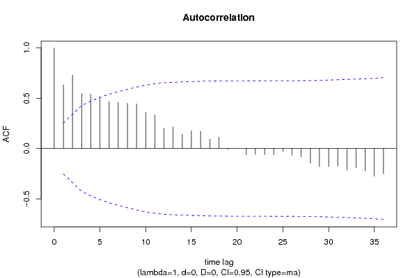
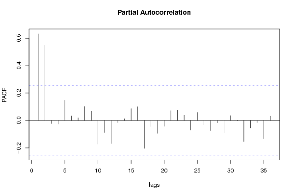
Title produced by software

(Partial) Autocorrelation Function

Date of computation

Fri, 27 Nov 2009 08:19:54 -0700

Cite this page as follows

Statistical Computations at FreeStatistics.org, Office for Research Development and Education, URL https://freestatistics.org/blog/index.php?v=date/2009/Nov/27/t1259335285v0rfwmrorr0dzfd.htm/, Retrieved Sat, 27 Apr 2024 13:38:32 +0000

Statistical Computations at FreeStatistics.org, Office for Research Development and Education, URL https://freestatistics.org/blog/index.php?pk=60896, Retrieved Sat, 27 Apr 2024 13:38:32 +0000

QR Codes:

Paste this QR Code to cite your computation.

Original text written by user:

IsPrivate?

No (this computation is public)

User-defined keywords

Estimated Impact

139

Family? (F = Feedback message, R = changed R code, M = changed R Module, P = changed Parameters, D = changed Data)

-     [Univariate Explorative Data Analysis] [Run Sequence gebo...] [2008-12-12 13:32:37] [76963dc1903f0f612b6153510a3818cf]
- R  D  [Univariate Explorative Data Analysis] [Run Sequence gebo...] [2008-12-17 12:14:40] [76963dc1903f0f612b6153510a3818cf]
-         [Univariate Explorative Data Analysis] [Run Sequence Plot...] [2008-12-22 18:19:51] [1ce0d16c8f4225c977b42c8fa93bc163]
- RMP       [(Partial) Autocorrelation Function] [Identifying Integ...] [2009-11-22 12:16:10] [b98453cac15ba1066b407e146608df68]
-    D        [(Partial) Autocorrelation Function] [ws 8] [2009-11-24 20:17:54] [b5908418e3090fddbd22f5f0f774653d]
-    D            [(Partial) Autocorrelation Function] [WS8 ACF] [2009-11-27 15:19:54] [557d56ec4b06cd0135c259898de8ce95] [Current]

Feedback Forum

Post a new message

Dataseries X:

Download CSV

Histogram

Boxplots

10284,5
12792
12823,61538
13845,66667
15335,63636
11188,5
13633,25
12298,46667
15353,63636
12696,15385
12213,93333
13683,72727
11214,14286
13950,23077
11179,13333
11801,875
11188,82353
16456,27273
11110,0625
16530,69231
10038,41176
11681,25
11148,88235
8631
9386,444444
9764,736842
12043,75
12948,06667
10987,125
11648,3125
10633,35294
10219,3
9037,6
10296,31579
11705,41176
10681,94444
9362,947368
11306,35294
10984,45
10062,61905
8118,583333
8867,48
8346,72
8529,307692
10697,18182
8591,84
8695,607143
8125,571429
7009,758621
7883,466667
7527,645161
6763,758621
6682,333333
7855,681818
6738,88
7895,434783
6361,884615
6935,956522
8344,454545
9107,944444

Summary of computational transaction
Raw Input	view raw input (R code)
Raw Output	view raw output of R engine
Computing time	2 seconds
R Server	'Gwilym Jenkins' @ 72.249.127.135

\begin{tabular}{lllllllll}
\hline
Summary of computational transaction \tabularnewline
Raw Input & view raw input (R code)  \tabularnewline
Raw Output & view raw output of R engine  \tabularnewline
Computing time & 2 seconds \tabularnewline
R Server & 'Gwilym Jenkins' @ 72.249.127.135 \tabularnewline
\hline
\end{tabular}
%Source: https://freestatistics.org/blog/index.php?pk=60896&T=0

[TABLE]
[ROW][C]Summary of computational transaction[/C][/ROW]
[ROW][C]Raw Input[/C][C]view raw input (R code) [/C][/ROW]
[ROW][C]Raw Output[/C][C]view raw output of R engine [/C][/ROW]
[ROW][C]Computing time[/C][C]2 seconds[/C][/ROW]
[ROW][C]R Server[/C][C]'Gwilym Jenkins' @ 72.249.127.135[/C][/ROW]
[/TABLE]
Source: https://freestatistics.org/blog/index.php?pk=60896&T=0

Globally Unique Identifier (entire table): ba.freestatistics.org/blog/index.php?pk=60896&T=0

As an alternative you can also use a QR Code:

The GUIDs for individual cells are displayed in the table below:

Summary of computational transaction
Raw Input	view raw input (R code)
Raw Output	view raw output of R engine
Computing time	2 seconds
R Server	'Gwilym Jenkins' @ 72.249.127.135

Autocorrelation Function
Time lag k	ACF(k)	T-STAT	P-value
1	0.632568	4.8999	4e-06
2	0.729162	5.6481	0
3	0.545761	4.2274	4.1e-05
4	0.542226	4.2001	4.5e-05
5	0.50682	3.9258	0.000113
6	0.465185	3.6033	0.00032
7	0.458129	3.5487	0.00038
8	0.449806	3.4842	0.000464
9	0.44426	3.4412	0.00053
10	0.360095	2.7893	0.003534
11	0.335324	2.5974	0.005899
12	0.203632	1.5773	0.059989
13	0.215965	1.6729	0.049781
14	0.140453	1.0879	0.140485
15	0.177946	1.3784	0.086604
16	0.171333	1.3271	0.094746
17	0.09243	0.716	0.238397
18	0.113228	0.8771	0.191976
19	-0.010321	-0.0799	0.468272
20	-0.002615	-0.0203	0.491953
21	-0.062579	-0.4847	0.314815
22	-0.05862	-0.4541	0.325709
23	-0.059967	-0.4645	0.321983
24	-0.061391	-0.4755	0.318067
25	-0.029952	-0.232	0.40866
26	-0.065299	-0.5058	0.307425
27	-0.082818	-0.6415	0.26182
28	-0.144011	-1.1155	0.134541
29	-0.18053	-1.3984	0.083573
30	-0.180121	-1.3952	0.084048
31	-0.173213	-1.3417	0.092375
32	-0.214891	-1.6645	0.05061
33	-0.19303	-1.4952	0.070051
34	-0.222623	-1.7244	0.04489
35	-0.275273	-2.1323	0.018544
36	-0.251755	-1.9501	0.027921

\begin{tabular}{lllllllll}
\hline
Autocorrelation Function \tabularnewline
Time lag k & ACF(k) & T-STAT & P-value \tabularnewline
1 & 0.632568 & 4.8999 & 4e-06 \tabularnewline
2 & 0.729162 & 5.6481 & 0 \tabularnewline
3 & 0.545761 & 4.2274 & 4.1e-05 \tabularnewline
4 & 0.542226 & 4.2001 & 4.5e-05 \tabularnewline
5 & 0.50682 & 3.9258 & 0.000113 \tabularnewline
6 & 0.465185 & 3.6033 & 0.00032 \tabularnewline
7 & 0.458129 & 3.5487 & 0.00038 \tabularnewline
8 & 0.449806 & 3.4842 & 0.000464 \tabularnewline
9 & 0.44426 & 3.4412 & 0.00053 \tabularnewline
10 & 0.360095 & 2.7893 & 0.003534 \tabularnewline
11 & 0.335324 & 2.5974 & 0.005899 \tabularnewline
12 & 0.203632 & 1.5773 & 0.059989 \tabularnewline
13 & 0.215965 & 1.6729 & 0.049781 \tabularnewline
14 & 0.140453 & 1.0879 & 0.140485 \tabularnewline
15 & 0.177946 & 1.3784 & 0.086604 \tabularnewline
16 & 0.171333 & 1.3271 & 0.094746 \tabularnewline
17 & 0.09243 & 0.716 & 0.238397 \tabularnewline
18 & 0.113228 & 0.8771 & 0.191976 \tabularnewline
19 & -0.010321 & -0.0799 & 0.468272 \tabularnewline
20 & -0.002615 & -0.0203 & 0.491953 \tabularnewline
21 & -0.062579 & -0.4847 & 0.314815 \tabularnewline
22 & -0.05862 & -0.4541 & 0.325709 \tabularnewline
23 & -0.059967 & -0.4645 & 0.321983 \tabularnewline
24 & -0.061391 & -0.4755 & 0.318067 \tabularnewline
25 & -0.029952 & -0.232 & 0.40866 \tabularnewline
26 & -0.065299 & -0.5058 & 0.307425 \tabularnewline
27 & -0.082818 & -0.6415 & 0.26182 \tabularnewline
28 & -0.144011 & -1.1155 & 0.134541 \tabularnewline
29 & -0.18053 & -1.3984 & 0.083573 \tabularnewline
30 & -0.180121 & -1.3952 & 0.084048 \tabularnewline
31 & -0.173213 & -1.3417 & 0.092375 \tabularnewline
32 & -0.214891 & -1.6645 & 0.05061 \tabularnewline
33 & -0.19303 & -1.4952 & 0.070051 \tabularnewline
34 & -0.222623 & -1.7244 & 0.04489 \tabularnewline
35 & -0.275273 & -2.1323 & 0.018544 \tabularnewline
36 & -0.251755 & -1.9501 & 0.027921 \tabularnewline
\hline
\end{tabular}
%Source: https://freestatistics.org/blog/index.php?pk=60896&T=1

[TABLE]
[ROW][C]Autocorrelation Function[/C][/ROW]
[ROW][C]Time lag k[/C][C]ACF(k)[/C][C]T-STAT[/C][C]P-value[/C][/ROW]
[ROW][C]1[/C][C]0.632568[/C][C]4.8999[/C][C]4e-06[/C][/ROW]
[ROW][C]2[/C][C]0.729162[/C][C]5.6481[/C][C]0[/C][/ROW]
[ROW][C]3[/C][C]0.545761[/C][C]4.2274[/C][C]4.1e-05[/C][/ROW]
[ROW][C]4[/C][C]0.542226[/C][C]4.2001[/C][C]4.5e-05[/C][/ROW]
[ROW][C]5[/C][C]0.50682[/C][C]3.9258[/C][C]0.000113[/C][/ROW]
[ROW][C]6[/C][C]0.465185[/C][C]3.6033[/C][C]0.00032[/C][/ROW]
[ROW][C]7[/C][C]0.458129[/C][C]3.5487[/C][C]0.00038[/C][/ROW]
[ROW][C]8[/C][C]0.449806[/C][C]3.4842[/C][C]0.000464[/C][/ROW]
[ROW][C]9[/C][C]0.44426[/C][C]3.4412[/C][C]0.00053[/C][/ROW]
[ROW][C]10[/C][C]0.360095[/C][C]2.7893[/C][C]0.003534[/C][/ROW]
[ROW][C]11[/C][C]0.335324[/C][C]2.5974[/C][C]0.005899[/C][/ROW]
[ROW][C]12[/C][C]0.203632[/C][C]1.5773[/C][C]0.059989[/C][/ROW]
[ROW][C]13[/C][C]0.215965[/C][C]1.6729[/C][C]0.049781[/C][/ROW]
[ROW][C]14[/C][C]0.140453[/C][C]1.0879[/C][C]0.140485[/C][/ROW]
[ROW][C]15[/C][C]0.177946[/C][C]1.3784[/C][C]0.086604[/C][/ROW]
[ROW][C]16[/C][C]0.171333[/C][C]1.3271[/C][C]0.094746[/C][/ROW]
[ROW][C]17[/C][C]0.09243[/C][C]0.716[/C][C]0.238397[/C][/ROW]
[ROW][C]18[/C][C]0.113228[/C][C]0.8771[/C][C]0.191976[/C][/ROW]
[ROW][C]19[/C][C]-0.010321[/C][C]-0.0799[/C][C]0.468272[/C][/ROW]
[ROW][C]20[/C][C]-0.002615[/C][C]-0.0203[/C][C]0.491953[/C][/ROW]
[ROW][C]21[/C][C]-0.062579[/C][C]-0.4847[/C][C]0.314815[/C][/ROW]
[ROW][C]22[/C][C]-0.05862[/C][C]-0.4541[/C][C]0.325709[/C][/ROW]
[ROW][C]23[/C][C]-0.059967[/C][C]-0.4645[/C][C]0.321983[/C][/ROW]
[ROW][C]24[/C][C]-0.061391[/C][C]-0.4755[/C][C]0.318067[/C][/ROW]
[ROW][C]25[/C][C]-0.029952[/C][C]-0.232[/C][C]0.40866[/C][/ROW]
[ROW][C]26[/C][C]-0.065299[/C][C]-0.5058[/C][C]0.307425[/C][/ROW]
[ROW][C]27[/C][C]-0.082818[/C][C]-0.6415[/C][C]0.26182[/C][/ROW]
[ROW][C]28[/C][C]-0.144011[/C][C]-1.1155[/C][C]0.134541[/C][/ROW]
[ROW][C]29[/C][C]-0.18053[/C][C]-1.3984[/C][C]0.083573[/C][/ROW]
[ROW][C]30[/C][C]-0.180121[/C][C]-1.3952[/C][C]0.084048[/C][/ROW]
[ROW][C]31[/C][C]-0.173213[/C][C]-1.3417[/C][C]0.092375[/C][/ROW]
[ROW][C]32[/C][C]-0.214891[/C][C]-1.6645[/C][C]0.05061[/C][/ROW]
[ROW][C]33[/C][C]-0.19303[/C][C]-1.4952[/C][C]0.070051[/C][/ROW]
[ROW][C]34[/C][C]-0.222623[/C][C]-1.7244[/C][C]0.04489[/C][/ROW]
[ROW][C]35[/C][C]-0.275273[/C][C]-2.1323[/C][C]0.018544[/C][/ROW]
[ROW][C]36[/C][C]-0.251755[/C][C]-1.9501[/C][C]0.027921[/C][/ROW]
[/TABLE]
Source: https://freestatistics.org/blog/index.php?pk=60896&T=1

Globally Unique Identifier (entire table): ba.freestatistics.org/blog/index.php?pk=60896&T=1

As an alternative you can also use a QR Code:

The GUIDs for individual cells are displayed in the table below:

Autocorrelation Function
Time lag k	ACF(k)	T-STAT	P-value
1	0.632568	4.8999	4e-06
2	0.729162	5.6481	0
3	0.545761	4.2274	4.1e-05
4	0.542226	4.2001	4.5e-05
5	0.50682	3.9258	0.000113
6	0.465185	3.6033	0.00032
7	0.458129	3.5487	0.00038
8	0.449806	3.4842	0.000464
9	0.44426	3.4412	0.00053
10	0.360095	2.7893	0.003534
11	0.335324	2.5974	0.005899
12	0.203632	1.5773	0.059989
13	0.215965	1.6729	0.049781
14	0.140453	1.0879	0.140485
15	0.177946	1.3784	0.086604
16	0.171333	1.3271	0.094746
17	0.09243	0.716	0.238397
18	0.113228	0.8771	0.191976
19	-0.010321	-0.0799	0.468272
20	-0.002615	-0.0203	0.491953
21	-0.062579	-0.4847	0.314815
22	-0.05862	-0.4541	0.325709
23	-0.059967	-0.4645	0.321983
24	-0.061391	-0.4755	0.318067
25	-0.029952	-0.232	0.40866
26	-0.065299	-0.5058	0.307425
27	-0.082818	-0.6415	0.26182
28	-0.144011	-1.1155	0.134541
29	-0.18053	-1.3984	0.083573
30	-0.180121	-1.3952	0.084048
31	-0.173213	-1.3417	0.092375
32	-0.214891	-1.6645	0.05061
33	-0.19303	-1.4952	0.070051
34	-0.222623	-1.7244	0.04489
35	-0.275273	-2.1323	0.018544
36	-0.251755	-1.9501	0.027921

Partial Autocorrelation Function
Time lag k	PACF(k)	T-STAT	P-value
1	0.632568	4.8999	4e-06
2	0.548497	4.2486	3.8e-05
3	-0.022542	-0.1746	0.430988
4	-0.0257	-0.1991	0.421439
5	0.148081	1.147	0.127961
6	0.034186	0.2648	0.396035
7	0.019867	0.1539	0.439108
8	0.101802	0.7886	0.216739
9	0.066887	0.5181	0.303146
10	-0.172472	-1.336	0.093304
11	-0.087596	-0.6785	0.250027
12	-0.168299	-1.3036	0.098669
13	-0.015599	-0.1208	0.452115
14	0.013375	0.1036	0.458916
15	0.086529	0.6703	0.252634
16	0.100305	0.777	0.220118
17	-0.203607	-1.5771	0.060011
18	-0.043999	-0.3408	0.367216
19	-0.094288	-0.7304	0.234008
20	-0.04253	-0.3294	0.371487
21	0.072272	0.5598	0.288843
22	0.074278	0.5754	0.283602
23	0.037598	0.2912	0.385938
24	-0.070511	-0.5462	0.293486
25	0.058195	0.4508	0.326886
26	-0.031515	-0.2441	0.403986
27	-0.074107	-0.574	0.284046
28	-0.016719	-0.1295	0.448696
29	-0.092039	-0.7129	0.239326
30	0.035615	0.2759	0.391798
31	-0.00328	-0.0254	0.489906
32	-0.153671	-1.1903	0.119302
33	-0.054296	-0.4206	0.337784
34	-0.015644	-0.1212	0.451976
35	-0.132669	-1.0276	0.15412
36	0.031561	0.2445	0.403852

\begin{tabular}{lllllllll}
\hline
Partial Autocorrelation Function \tabularnewline
Time lag k & PACF(k) & T-STAT & P-value \tabularnewline
1 & 0.632568 & 4.8999 & 4e-06 \tabularnewline
2 & 0.548497 & 4.2486 & 3.8e-05 \tabularnewline
3 & -0.022542 & -0.1746 & 0.430988 \tabularnewline
4 & -0.0257 & -0.1991 & 0.421439 \tabularnewline
5 & 0.148081 & 1.147 & 0.127961 \tabularnewline
6 & 0.034186 & 0.2648 & 0.396035 \tabularnewline
7 & 0.019867 & 0.1539 & 0.439108 \tabularnewline
8 & 0.101802 & 0.7886 & 0.216739 \tabularnewline
9 & 0.066887 & 0.5181 & 0.303146 \tabularnewline
10 & -0.172472 & -1.336 & 0.093304 \tabularnewline
11 & -0.087596 & -0.6785 & 0.250027 \tabularnewline
12 & -0.168299 & -1.3036 & 0.098669 \tabularnewline
13 & -0.015599 & -0.1208 & 0.452115 \tabularnewline
14 & 0.013375 & 0.1036 & 0.458916 \tabularnewline
15 & 0.086529 & 0.6703 & 0.252634 \tabularnewline
16 & 0.100305 & 0.777 & 0.220118 \tabularnewline
17 & -0.203607 & -1.5771 & 0.060011 \tabularnewline
18 & -0.043999 & -0.3408 & 0.367216 \tabularnewline
19 & -0.094288 & -0.7304 & 0.234008 \tabularnewline
20 & -0.04253 & -0.3294 & 0.371487 \tabularnewline
21 & 0.072272 & 0.5598 & 0.288843 \tabularnewline
22 & 0.074278 & 0.5754 & 0.283602 \tabularnewline
23 & 0.037598 & 0.2912 & 0.385938 \tabularnewline
24 & -0.070511 & -0.5462 & 0.293486 \tabularnewline
25 & 0.058195 & 0.4508 & 0.326886 \tabularnewline
26 & -0.031515 & -0.2441 & 0.403986 \tabularnewline
27 & -0.074107 & -0.574 & 0.284046 \tabularnewline
28 & -0.016719 & -0.1295 & 0.448696 \tabularnewline
29 & -0.092039 & -0.7129 & 0.239326 \tabularnewline
30 & 0.035615 & 0.2759 & 0.391798 \tabularnewline
31 & -0.00328 & -0.0254 & 0.489906 \tabularnewline
32 & -0.153671 & -1.1903 & 0.119302 \tabularnewline
33 & -0.054296 & -0.4206 & 0.337784 \tabularnewline
34 & -0.015644 & -0.1212 & 0.451976 \tabularnewline
35 & -0.132669 & -1.0276 & 0.15412 \tabularnewline
36 & 0.031561 & 0.2445 & 0.403852 \tabularnewline
\hline
\end{tabular}
%Source: https://freestatistics.org/blog/index.php?pk=60896&T=2

[TABLE]
[ROW][C]Partial Autocorrelation Function[/C][/ROW]
[ROW][C]Time lag k[/C][C]PACF(k)[/C][C]T-STAT[/C][C]P-value[/C][/ROW]
[ROW][C]1[/C][C]0.632568[/C][C]4.8999[/C][C]4e-06[/C][/ROW]
[ROW][C]2[/C][C]0.548497[/C][C]4.2486[/C][C]3.8e-05[/C][/ROW]
[ROW][C]3[/C][C]-0.022542[/C][C]-0.1746[/C][C]0.430988[/C][/ROW]
[ROW][C]4[/C][C]-0.0257[/C][C]-0.1991[/C][C]0.421439[/C][/ROW]
[ROW][C]5[/C][C]0.148081[/C][C]1.147[/C][C]0.127961[/C][/ROW]
[ROW][C]6[/C][C]0.034186[/C][C]0.2648[/C][C]0.396035[/C][/ROW]
[ROW][C]7[/C][C]0.019867[/C][C]0.1539[/C][C]0.439108[/C][/ROW]
[ROW][C]8[/C][C]0.101802[/C][C]0.7886[/C][C]0.216739[/C][/ROW]
[ROW][C]9[/C][C]0.066887[/C][C]0.5181[/C][C]0.303146[/C][/ROW]
[ROW][C]10[/C][C]-0.172472[/C][C]-1.336[/C][C]0.093304[/C][/ROW]
[ROW][C]11[/C][C]-0.087596[/C][C]-0.6785[/C][C]0.250027[/C][/ROW]
[ROW][C]12[/C][C]-0.168299[/C][C]-1.3036[/C][C]0.098669[/C][/ROW]
[ROW][C]13[/C][C]-0.015599[/C][C]-0.1208[/C][C]0.452115[/C][/ROW]
[ROW][C]14[/C][C]0.013375[/C][C]0.1036[/C][C]0.458916[/C][/ROW]
[ROW][C]15[/C][C]0.086529[/C][C]0.6703[/C][C]0.252634[/C][/ROW]
[ROW][C]16[/C][C]0.100305[/C][C]0.777[/C][C]0.220118[/C][/ROW]
[ROW][C]17[/C][C]-0.203607[/C][C]-1.5771[/C][C]0.060011[/C][/ROW]
[ROW][C]18[/C][C]-0.043999[/C][C]-0.3408[/C][C]0.367216[/C][/ROW]
[ROW][C]19[/C][C]-0.094288[/C][C]-0.7304[/C][C]0.234008[/C][/ROW]
[ROW][C]20[/C][C]-0.04253[/C][C]-0.3294[/C][C]0.371487[/C][/ROW]
[ROW][C]21[/C][C]0.072272[/C][C]0.5598[/C][C]0.288843[/C][/ROW]
[ROW][C]22[/C][C]0.074278[/C][C]0.5754[/C][C]0.283602[/C][/ROW]
[ROW][C]23[/C][C]0.037598[/C][C]0.2912[/C][C]0.385938[/C][/ROW]
[ROW][C]24[/C][C]-0.070511[/C][C]-0.5462[/C][C]0.293486[/C][/ROW]
[ROW][C]25[/C][C]0.058195[/C][C]0.4508[/C][C]0.326886[/C][/ROW]
[ROW][C]26[/C][C]-0.031515[/C][C]-0.2441[/C][C]0.403986[/C][/ROW]
[ROW][C]27[/C][C]-0.074107[/C][C]-0.574[/C][C]0.284046[/C][/ROW]
[ROW][C]28[/C][C]-0.016719[/C][C]-0.1295[/C][C]0.448696[/C][/ROW]
[ROW][C]29[/C][C]-0.092039[/C][C]-0.7129[/C][C]0.239326[/C][/ROW]
[ROW][C]30[/C][C]0.035615[/C][C]0.2759[/C][C]0.391798[/C][/ROW]
[ROW][C]31[/C][C]-0.00328[/C][C]-0.0254[/C][C]0.489906[/C][/ROW]
[ROW][C]32[/C][C]-0.153671[/C][C]-1.1903[/C][C]0.119302[/C][/ROW]
[ROW][C]33[/C][C]-0.054296[/C][C]-0.4206[/C][C]0.337784[/C][/ROW]
[ROW][C]34[/C][C]-0.015644[/C][C]-0.1212[/C][C]0.451976[/C][/ROW]
[ROW][C]35[/C][C]-0.132669[/C][C]-1.0276[/C][C]0.15412[/C][/ROW]
[ROW][C]36[/C][C]0.031561[/C][C]0.2445[/C][C]0.403852[/C][/ROW]
[/TABLE]
Source: https://freestatistics.org/blog/index.php?pk=60896&T=2

Globally Unique Identifier (entire table): ba.freestatistics.org/blog/index.php?pk=60896&T=2

As an alternative you can also use a QR Code:

The GUIDs for individual cells are displayed in the table below:

Partial Autocorrelation Function
Time lag k	PACF(k)	T-STAT	P-value
1	0.632568	4.8999	4e-06
2	0.548497	4.2486	3.8e-05
3	-0.022542	-0.1746	0.430988
4	-0.0257	-0.1991	0.421439
5	0.148081	1.147	0.127961
6	0.034186	0.2648	0.396035
7	0.019867	0.1539	0.439108
8	0.101802	0.7886	0.216739
9	0.066887	0.5181	0.303146
10	-0.172472	-1.336	0.093304
11	-0.087596	-0.6785	0.250027
12	-0.168299	-1.3036	0.098669
13	-0.015599	-0.1208	0.452115
14	0.013375	0.1036	0.458916
15	0.086529	0.6703	0.252634
16	0.100305	0.777	0.220118
17	-0.203607	-1.5771	0.060011
18	-0.043999	-0.3408	0.367216
19	-0.094288	-0.7304	0.234008
20	-0.04253	-0.3294	0.371487
21	0.072272	0.5598	0.288843
22	0.074278	0.5754	0.283602
23	0.037598	0.2912	0.385938
24	-0.070511	-0.5462	0.293486
25	0.058195	0.4508	0.326886
26	-0.031515	-0.2441	0.403986
27	-0.074107	-0.574	0.284046
28	-0.016719	-0.1295	0.448696
29	-0.092039	-0.7129	0.239326
30	0.035615	0.2759	0.391798
31	-0.00328	-0.0254	0.489906
32	-0.153671	-1.1903	0.119302
33	-0.054296	-0.4206	0.337784
34	-0.015644	-0.1212	0.451976
35	-0.132669	-1.0276	0.15412
36	0.031561	0.2445	0.403852

Figure 1

PNG link

Postscript link

PDF link

Figure 2

PNG link

Postscript link

PDF link

Parameters (Session):

par1 = 36 ; par2 = 1 ; par3 = 0 ; par4 = 0 ; par5 = 12 ; par6 = MA ; par7 = 0.95 ;

Parameters (R input):

par1 = 36 ; par2 = 1 ; par3 = 0 ; par4 = 0 ; par5 = 12 ; par6 = MA ; par7 = 0.95 ;

R code (references can be found in the software module):

if (par1 == 'Default') {
par1 = 10*log10(length(x))
} else {
par1 <- as.numeric(par1)
}
par2 <- as.numeric(par2)
par3 <- as.numeric(par3)
par4 <- as.numeric(par4)
par5 <- as.numeric(par5)
if (par6 == 'White Noise') par6 <- 'white' else par6 <- 'ma'
par7 <- as.numeric(par7)
if (par2 == 0) {
x <- log(x)
} else {
x <- (x ^ par2 - 1) / par2
}
if (par3 > 0) x <- diff(x,lag=1,difference=par3)
if (par4 > 0) x <- diff(x,lag=par5,difference=par4)
bitmap(file='pic1.png')
racf <- acf(x, par1, main='Autocorrelation', xlab='time lag', ylab='ACF', ci.type=par6, ci=par7, sub=paste('(lambda=',par2,', d=',par3,', D=',par4,', CI=', par7, ', CI type=',par6,')',sep=''))
dev.off()
bitmap(file='pic2.png')
rpacf <- pacf(x,par1,main='Partial Autocorrelation',xlab='lags',ylab='PACF')
dev.off()
(myacf <- c(racf$acf))
(mypacf <- c(rpacf$acf))
lengthx <- length(x)
sqrtn <- sqrt(lengthx)
load(file='createtable')
a<-table.start()
a<-table.row.start(a)
a<-table.element(a,'Autocorrelation Function',4,TRUE)
a<-table.row.end(a)
a<-table.row.start(a)
a<-table.element(a,'Time lag k',header=TRUE)
a<-table.element(a,hyperlink('basics.htm','ACF(k)','click here for more information about the Autocorrelation Function'),header=TRUE)
a<-table.element(a,'T-STAT',header=TRUE)
a<-table.element(a,'P-value',header=TRUE)
a<-table.row.end(a)
for (i in 2:(par1+1)) {
a<-table.row.start(a)
a<-table.element(a,i-1,header=TRUE)
a<-table.element(a,round(myacf[i],6))
mytstat <- myacf[i]*sqrtn
a<-table.element(a,round(mytstat,4))
a<-table.element(a,round(1-pt(abs(mytstat),lengthx),6))
a<-table.row.end(a)
}
a<-table.end(a)
table.save(a,file='mytable.tab')
a<-table.start()
a<-table.row.start(a)
a<-table.element(a,'Partial Autocorrelation Function',4,TRUE)
a<-table.row.end(a)
a<-table.row.start(a)
a<-table.element(a,'Time lag k',header=TRUE)
a<-table.element(a,hyperlink('basics.htm','PACF(k)','click here for more information about the Partial Autocorrelation Function'),header=TRUE)
a<-table.element(a,'T-STAT',header=TRUE)
a<-table.element(a,'P-value',header=TRUE)
a<-table.row.end(a)
for (i in 1:par1) {
a<-table.row.start(a)
a<-table.element(a,i,header=TRUE)
a<-table.element(a,round(mypacf[i],6))
mytstat <- mypacf[i]*sqrtn
a<-table.element(a,round(mytstat,4))
a<-table.element(a,round(1-pt(abs(mytstat),lengthx),6))
a<-table.row.end(a)
}
a<-table.end(a)
table.save(a,file='mytable1.tab')

Free Statistics

Description of Statistical Computation

Tree of Dependent Computations

Dataset

Tables (Output of Computation)

Figures (Output of Computation)

Input Parameters & R Code