Blog & Share Statistical Computations at FreeStatistics.org

Home » date » 2009 » Nov » 18 »

*The author of this computation has been verified*

R Software Module: /rwasp_multipleregression.wasp (opens new window with default values)

Title produced by software: Multiple Regression

Date of computation: Wed, 18 Nov 2009 11:37:15 -0700

Cite this page as follows:

Statistical Computations at FreeStatistics.org, Office for Research Development and Education, URL http://www.freestatistics.org/blog/date/2009/Nov/18/t1258569513c4yozh6xbbjxmqj.htm/, Retrieved Wed, 18 Nov 2009 19:38:45 +0100

BibTeX entries for LaTeX users:

@Manual{KEY,
    author = {{YOUR NAME}},
    publisher = {Office for Research Development and Education},
    title = {Statistical Computations at FreeStatistics.org, URL http://www.freestatistics.org/blog/date/2009/Nov/18/t1258569513c4yozh6xbbjxmqj.htm/},
    year = {2009},
}
@Manual{R,
    title = {R: A Language and Environment for Statistical Computing},
    author = {{R Development Core Team}},
    organization = {R Foundation for Statistical Computing},
    address = {Vienna, Austria},
    year = {2009},
    note = {{ISBN} 3-900051-07-0},
    url = {http://www.R-project.org},
}

Original text written by user:

IsPrivate?

No (this computation is public)

User-defined keywords:

Dataseries X:

» Textbox « » Textfile « » CSV «

90398 562000 90269 561000 90390 555000 88219 544000 87032 537000 87175 543000 92603 594000 93571 611000 94118 613000 92159 611000 89528 594000 89955 595000 89587 591000 89488 589000 88521 584000 86587 573000 85159 567000 84915 569000 91378 621000 92729 629000 92194 628000 89664 612000 86285 595000 86858 597000 87184 593000 86629 590000 85220 580000 84816 574000 84831 573000 84957 573000 90951 620000 92134 626000 91790 620000 86625 588000 83324 566000 82719 557000 83614 561000 81640 549000 78665 532000 77828 526000 75728 511000 72187 499000 79357 555000 81329 565000 77304 542000 75576 527000 72932 510000 74291 514000 74988 517000 73302 508000 70483 493000 69848 490000 66466 469000 67610 478000 75091 528000 76207 534000 73454 518000 72008 506000 71362 502000 74250 516000

Output produced by software:

Enter (or paste) a matrix (table) containing all data (time) series. Every column represents a different variable and must be delimited by a space or Tab. Every row represents a period in time (or category) and must be delimited by hard returns. The easiest way to enter data is to copy and paste a block of spreadsheet cells. Please, do not use commas or spaces to seperate groups of digits!

Summary of computational transaction
Raw Input	view raw input (R code)
Raw Output	view raw output of R engine
Computing time	3 seconds
R Server	'Gwilym Jenkins' @ 72.249.127.135

Multiple Linear Regression - Estimated Regression Equation

Y[t] = -20578.3075841541 + 0.183866332465193X[t] + 1884.80300781325M1[t] + 1989.08120312530M2[t] + 2328.26432725635M3[t] + 2492.67518749878M4[t] + 2714.93851215070M5[t] + 2056.67217968551M6[t] -850.08404253236M7[t] -1260.42756770517M8[t] -1064.40384201148M9[t] -798.462322047506M10[t] -487.120802083538M11[t] + e[t]

Multiple Linear Regression - Ordinary Least Squares
Variable	Parameter	S.D.	T-STAT H0: parameter = 0	2-tail p-value	1-tail p-value
(Intercept)	-20578.3075841541	5588.045948	-3.6826	0.000595	0.000298
X	0.183866332465193	0.009798	18.7652	0	0
M1	1884.80300781325	1773.558784	1.0627	0.293337	0.146669
M2	1989.08120312530	1771.716272	1.1227	0.267273	0.133637
M3	2328.26432725635	1772.692468	1.3134	0.195422	0.097711
M4	2492.67518749878	1776.975523	1.4028	0.167259	0.08363
M5	2714.93851215070	1787.426116	1.5189	0.135484	0.067742
M6	2056.67217968551	1786.141948	1.1515	0.255367	0.127683
M7	-850.08404253236	1792.186141	-0.4743	0.637462	0.318731
M8	-1260.42756770517	1808.477395	-0.697	0.489264	0.244632
M9	-1064.40384201148	1793.089085	-0.5936	0.555616	0.277808
M10	-798.462322047506	1775.938974	-0.4496	0.655066	0.327533
M11	-487.120802083538	1771.521186	-0.275	0.784542	0.392271

Multiple Linear Regression - Regression Statistics
Multiple R	0.945772715791592
R-squared	0.894486029935803
Adjusted R-squared	0.867546292898136
F-TEST (value)	33.2032205320018
F-TEST (DF numerator)	12
F-TEST (DF denominator)	47
p-value	0
Multiple Linear Regression - Residual Statistics
Residual Standard Deviation	2800.77414274199
Sum Squared Residuals	368683782.536650

Multiple Linear Regression - Actuals, Interpolation, and Residuals
Time or Index	Actuals	Interpolation Forecast	Residuals Prediction Error
1	90398	84639.3742690975	5758.62573090246
2	90269	84559.7861319443	5709.21386805568
3	90390	83795.7712612842	6594.2287387158
4	88219	81937.6524644095	6281.3475355905
5	87032	80872.8514618051	6159.14853819492
6	87175	81317.783124131	5857.21687586895
7	92603	87788.209857638	4814.79014236200
8	93571	90503.5939843735	3067.40601562653
9	94118	91067.3503749975	3050.64962500245
10	92159	90965.5592300311	1193.44076996886
11	89528	88151.1730980868	1376.82690191317
12	89955	88822.1602326356	1132.83976736444
13	89587	89971.497910588	-384.49791058803
14	89488	89708.0434409697	-220.043440969703
15	88521	89127.8949027748	-606.894902774786
16	86587	87269.7761059001	-682.776105900093
17	85159	86388.8414357609	-1229.84143576086
18	84915	86098.307768226	-1183.30776822606
19	91378	92752.6008341982	-1374.60083419821
20	92729	93813.187968747	-1084.18796874694
21	92194	93825.3453619754	-1631.34536197544
22	89664	91149.4255624963	-1485.42556249633
23	86285	88335.039430552	-2050.03943055202
24	86858	89189.892897566	-2331.89289756594
25	87184	90339.2305755184	-3155.23057551842
26	86629	89891.9097734349	-3262.90977343490
27	85220	88392.429572914	-3172.42957291401
28	84816	87453.6424383653	-2637.64243836529
29	84831	87492.039430552	-2661.03943055202
30	84957	86833.7730980868	-1876.77309808683
31	90951	92568.734501733	-1617.73450173302
32	92134	93261.5889713514	-1127.58897135136
33	91790	92354.4147022539	-564.414702253901
34	86625	86736.6335833317	-111.633583331701
35	83324	83002.9157890614	321.08421093857
36	82719	81835.2395989582	883.760401041769
37	83614	84455.5079366322	-841.507936632245
38	81640	82353.390142362	-713.390142361991
39	78665	79566.8456145848	-901.845614584762
40	77828	78628.058480036	-800.058480036032
41	75728	76092.32681771	-364.326817710067
42	72187	73227.6644956626	-1040.66449566256
43	79357	80617.4228914955	-1260.42289149548
44	81329	82045.7426909746	-716.742690974601
45	77304	78012.8407699689	-708.840769968862
46	75576	75520.787302955	55.2126970450593
47	72932	72706.4011710106	225.598828989367
48	74291	73928.987302955	362.012697045059
49	74988	76365.3893081638	-1377.38930816376
50	73302	74814.8705112891	-1512.87051128909
51	70483	72396.0586484422	-1913.05864844224
52	69848	72008.8705112891	-2160.87051128909
53	66466	68369.940854172	-1903.94085417197
54	67610	69366.4715138935	-1756.47151389351
55	75091	75653.0319149353	-562.03191493528
56	76207	76345.8863845536	-138.886384553624
57	73454	73600.0487908042	-146.048790804236
58	72008	71659.5943211859	348.405678814108
59	71362	71235.4705112891	126.529488710910
60	74250	74296.7199678853	-46.7199678853268

Goldfeld-Quandt test for Heteroskedasticity
p-values	Alternative Hypothesis
breakpoint index	greater	2-sided	less
16	0.131398066233327	0.262796132466653	0.868601933766673
17	0.0784524735844108	0.156904947168822	0.921547526415589
18	0.105351248455518	0.210702496911035	0.894648751544482
19	0.052902886994351	0.105805773988702	0.94709711300565
20	0.023686069232098	0.047372138464196	0.976313930767902
21	0.0425023409172739	0.0850046818345477	0.957497659082726
22	0.333949708607858	0.667899417215716	0.666050291392142
23	0.796940104601533	0.406119790796935	0.203059895398467
24	0.962328956232864	0.0753420875342728	0.0376710437671364
25	0.983116040891941	0.0337679182161172	0.0168839591080586
26	0.996274252704732	0.00745149459053665	0.00372574729526832
27	0.999687138982858	0.00062572203428354	0.00031286101714177
28	0.999667388272131	0.000665223455737706	0.000332611727868853
29	0.999803587733717	0.000392824532566522	0.000196412266283261
30	0.999578454283396	0.000843091433207404	0.000421545716603702
31	0.999379940615318	0.00124011876936455	0.000620059384682276
32	0.99933630990578	0.00132738018844049	0.000663690094220245
33	0.99913405822839	0.00173188354322095	0.000865941771610474
34	0.999961970310798	7.60593784031995e-05	3.80296892015998e-05
35	0.999988813521417	2.23729571668393e-05	1.11864785834197e-05
36	0.99999067395664	1.86520867192285e-05	9.32604335961424e-06
37	0.999983336178172	3.33276436558205e-05	1.66638218279103e-05
38	0.99997187072549	5.62585490195347e-05	2.81292745097674e-05
39	0.999954465947775	9.10681044495212e-05	4.55340522247606e-05
40	0.999933184975565	0.000133630048869688	6.6815024434844e-05
41	0.99998914615701	2.17076859795375e-05	1.08538429897688e-05
42	0.999998888918517	2.2221629659937e-06	1.11108148299685e-06
43	0.999984040775214	3.19184495716426e-05	1.59592247858213e-05
44	0.999687176493519	0.000625647012962782	0.000312823506481391

Meta Analysis of Goldfeld-Quandt test for Heteroskedasticity
Description	# significant tests	% significant tests	OK/NOK
1% type I error level	19	0.655172413793103	NOK
5% type I error level	21	0.724137931034483	NOK
10% type I error level	23	0.793103448275862	NOK

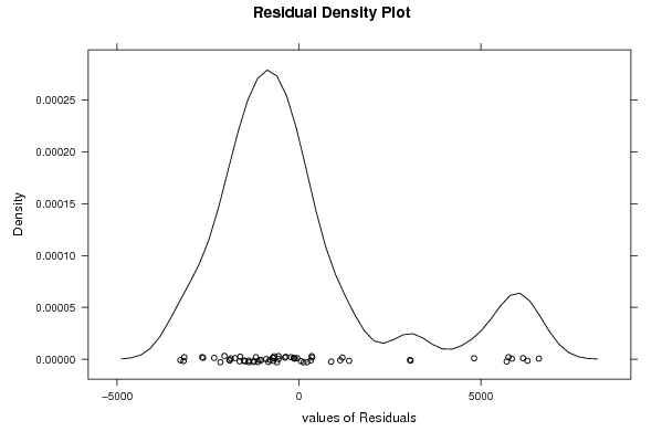
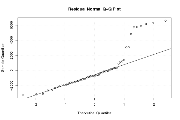
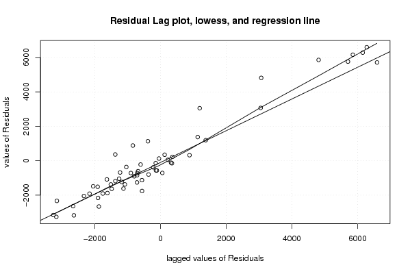
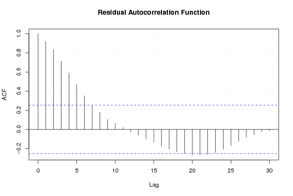
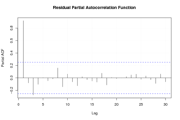
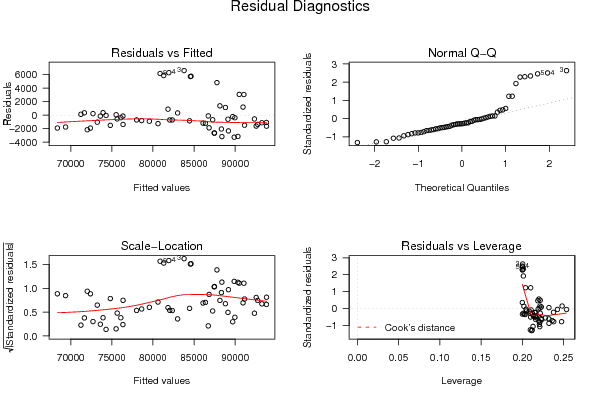
Charts produced by software:

http://www.freestatistics.org/blog/date/2009/Nov/18/t1258569513c4yozh6xbbjxmqj/1010z01258569430.png (open in new window)

http://www.freestatistics.org/blog/date/2009/Nov/18/t1258569513c4yozh6xbbjxmqj/1010z01258569430.ps (open in new window)

http://www.freestatistics.org/blog/date/2009/Nov/18/t1258569513c4yozh6xbbjxmqj/1t24u1258569430.png (open in new window)

http://www.freestatistics.org/blog/date/2009/Nov/18/t1258569513c4yozh6xbbjxmqj/1t24u1258569430.ps (open in new window)

http://www.freestatistics.org/blog/date/2009/Nov/18/t1258569513c4yozh6xbbjxmqj/23bdo1258569430.png (open in new window)

http://www.freestatistics.org/blog/date/2009/Nov/18/t1258569513c4yozh6xbbjxmqj/23bdo1258569430.ps (open in new window)

http://www.freestatistics.org/blog/date/2009/Nov/18/t1258569513c4yozh6xbbjxmqj/3077n1258569430.png (open in new window)

http://www.freestatistics.org/blog/date/2009/Nov/18/t1258569513c4yozh6xbbjxmqj/3077n1258569430.ps (open in new window)

http://www.freestatistics.org/blog/date/2009/Nov/18/t1258569513c4yozh6xbbjxmqj/4rri61258569430.png (open in new window)

http://www.freestatistics.org/blog/date/2009/Nov/18/t1258569513c4yozh6xbbjxmqj/4rri61258569430.ps (open in new window)

http://www.freestatistics.org/blog/date/2009/Nov/18/t1258569513c4yozh6xbbjxmqj/50s1g1258569430.png (open in new window)

http://www.freestatistics.org/blog/date/2009/Nov/18/t1258569513c4yozh6xbbjxmqj/50s1g1258569430.ps (open in new window)

http://www.freestatistics.org/blog/date/2009/Nov/18/t1258569513c4yozh6xbbjxmqj/6ga4u1258569430.png (open in new window)

http://www.freestatistics.org/blog/date/2009/Nov/18/t1258569513c4yozh6xbbjxmqj/6ga4u1258569430.ps (open in new window)

http://www.freestatistics.org/blog/date/2009/Nov/18/t1258569513c4yozh6xbbjxmqj/7mro71258569430.png (open in new window)

http://www.freestatistics.org/blog/date/2009/Nov/18/t1258569513c4yozh6xbbjxmqj/7mro71258569430.ps (open in new window)

http://www.freestatistics.org/blog/date/2009/Nov/18/t1258569513c4yozh6xbbjxmqj/85r7x1258569430.png (open in new window)

http://www.freestatistics.org/blog/date/2009/Nov/18/t1258569513c4yozh6xbbjxmqj/85r7x1258569430.ps (open in new window)

http://www.freestatistics.org/blog/date/2009/Nov/18/t1258569513c4yozh6xbbjxmqj/95hd51258569430.png (open in new window)

http://www.freestatistics.org/blog/date/2009/Nov/18/t1258569513c4yozh6xbbjxmqj/95hd51258569430.ps (open in new window)

Parameters (Session):

par1 = 2 ; par2 = Do not include Seasonal Dummies ; par3 = Linear Trend ;

Parameters (R input):

par1 = 1 ; par2 = Include Monthly Dummies ; par3 = No Linear Trend ;

R code (references can be found in the software module):

library(lattice)

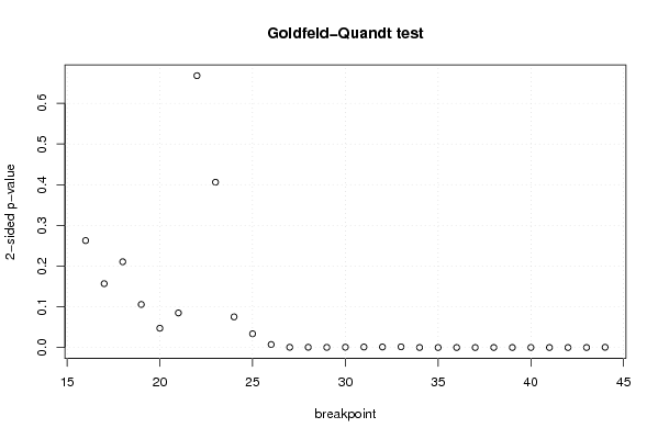
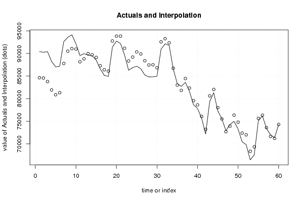
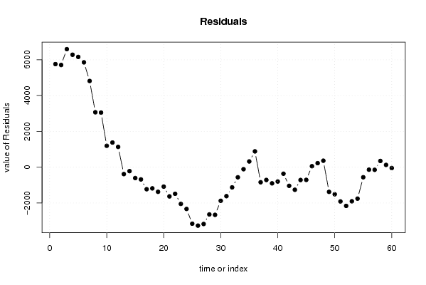
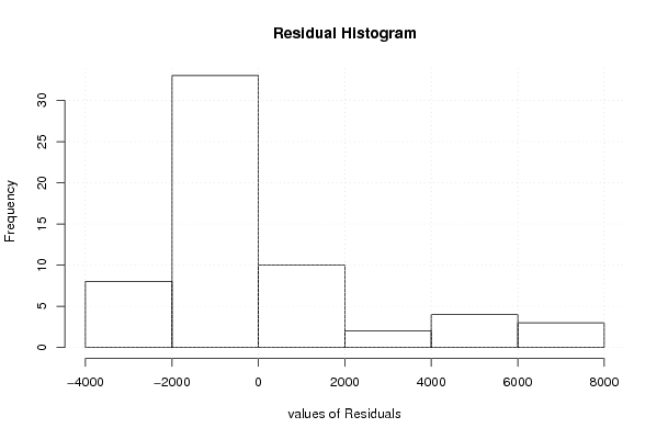
library(lmtest)

n25 <- 25 #minimum number of obs. for Goldfeld-Quandt test

par1 <- as.numeric(par1)

x <- t(y)

k <- length(x[1,])

n <- length(x[,1])

x1 <- cbind(x[,par1], x[,1:k!=par1])

mycolnames <- c(colnames(x)[par1], colnames(x)[1:k!=par1])

colnames(x1) <- mycolnames #colnames(x)[par1]

x <- x1

if (par3 == 'First Differences'){

x2 <- array(0, dim=c(n-1,k), dimnames=list(1:(n-1), paste('(1-B)',colnames(x),sep='')))

for (i in 1:n-1) {

for (j in 1:k) {

x2[i,j] <- x[i+1,j] - x[i,j]

}

}

x <- x2

}

if (par2 == 'Include Monthly Dummies'){

x2 <- array(0, dim=c(n,11), dimnames=list(1:n, paste('M', seq(1:11), sep ='')))

for (i in 1:11){

x2[seq(i,n,12),i] <- 1

}

x <- cbind(x, x2)

}

if (par2 == 'Include Quarterly Dummies'){

x2 <- array(0, dim=c(n,3), dimnames=list(1:n, paste('Q', seq(1:3), sep ='')))

for (i in 1:3){

x2[seq(i,n,4),i] <- 1

}

x <- cbind(x, x2)

}

k <- length(x[1,])

if (par3 == 'Linear Trend'){

x <- cbind(x, c(1:n))

colnames(x)[k+1] <- 't'

}

x

k <- length(x[1,])

df <- as.data.frame(x)

(mylm <- lm(df))

(mysum <- summary(mylm))

if (n > n25) {

kp3 <- k + 3

nmkm3 <- n - k - 3

gqarr <- array(NA, dim=c(nmkm3-kp3+1,3))

numgqtests <- 0

numsignificant1 <- 0

numsignificant5 <- 0

numsignificant10 <- 0

for (mypoint in kp3:nmkm3) {

j <- 0

numgqtests <- numgqtests + 1

for (myalt in c('greater', 'two.sided', 'less')) {

j <- j + 1

gqarr[mypoint-kp3+1,j] <- gqtest(mylm, point=mypoint, alternative=myalt)$p.value

}

if (gqarr[mypoint-kp3+1,2] < 0.01) numsignificant1 <- numsignificant1 + 1

if (gqarr[mypoint-kp3+1,2] < 0.05) numsignificant5 <- numsignificant5 + 1

if (gqarr[mypoint-kp3+1,2] < 0.10) numsignificant10 <- numsignificant10 + 1

}

gqarr

}

bitmap(file='test0.png')

plot(x[,1], type='l', main='Actuals and Interpolation', ylab='value of Actuals and Interpolation (dots)', xlab='time or index')

points(x[,1]-mysum$resid)

grid()

dev.off()

bitmap(file='test1.png')

plot(mysum$resid, type='b', pch=19, main='Residuals', ylab='value of Residuals', xlab='time or index')

grid()

dev.off()

bitmap(file='test2.png')

hist(mysum$resid, main='Residual Histogram', xlab='values of Residuals')

grid()

dev.off()

bitmap(file='test3.png')

densityplot(~mysum$resid,col='black',main='Residual Density Plot', xlab='values of Residuals')

dev.off()

bitmap(file='test4.png')

qqnorm(mysum$resid, main='Residual Normal Q-Q Plot')

qqline(mysum$resid)

grid()

dev.off()

(myerror <- as.ts(mysum$resid))

bitmap(file='test5.png')

dum <- cbind(lag(myerror,k=1),myerror)

dum

dum1 <- dum[2:length(myerror),]

dum1

z <- as.data.frame(dum1)

z

plot(z,main=paste('Residual Lag plot, lowess, and regression line'), ylab='values of Residuals', xlab='lagged values of Residuals')

lines(lowess(z))

abline(lm(z))

grid()

dev.off()

bitmap(file='test6.png')

acf(mysum$resid, lag.max=length(mysum$resid)/2, main='Residual Autocorrelation Function')

grid()

dev.off()

bitmap(file='test7.png')

pacf(mysum$resid, lag.max=length(mysum$resid)/2, main='Residual Partial Autocorrelation Function')

grid()

dev.off()

bitmap(file='test8.png')

opar <- par(mfrow = c(2,2), oma = c(0, 0, 1.1, 0))

plot(mylm, las = 1, sub='Residual Diagnostics')

par(opar)

dev.off()

if (n > n25) {

bitmap(file='test9.png')

plot(kp3:nmkm3,gqarr[,2], main='Goldfeld-Quandt test',ylab='2-sided p-value',xlab='breakpoint')

grid()

dev.off()

}

load(file='createtable')

a<-table.start()

a<-table.row.start(a)

a<-table.element(a, 'Multiple Linear Regression - Estimated Regression Equation', 1, TRUE)

a<-table.row.end(a)

myeq <- colnames(x)[1]

myeq <- paste(myeq, '[t] = ', sep='')

for (i in 1:k){

if (mysum$coefficients[i,1] > 0) myeq <- paste(myeq, '+', '')

myeq <- paste(myeq, mysum$coefficients[i,1], sep=' ')

if (rownames(mysum$coefficients)[i] != '(Intercept)') {

myeq <- paste(myeq, rownames(mysum$coefficients)[i], sep='')

if (rownames(mysum$coefficients)[i] != 't') myeq <- paste(myeq, '[t]', sep='')

}

}

myeq <- paste(myeq, ' + e[t]')

a<-table.row.start(a)

a<-table.element(a, myeq)

a<-table.row.end(a)

a<-table.end(a)

table.save(a,file='mytable1.tab')

a<-table.start()

a<-table.row.start(a)

a<-table.element(a,hyperlink('http://www.xycoon.com/ols1.htm','Multiple Linear Regression - Ordinary Least Squares',''), 6, TRUE)

a<-table.row.end(a)

a<-table.row.start(a)

a<-table.element(a,'Variable',header=TRUE)

a<-table.element(a,'Parameter',header=TRUE)

a<-table.element(a,'S.D.',header=TRUE)

a<-table.element(a,'T-STAT<br />H0: parameter = 0',header=TRUE)

a<-table.element(a,'2-tail p-value',header=TRUE)

a<-table.element(a,'1-tail p-value',header=TRUE)

a<-table.row.end(a)

for (i in 1:k){

a<-table.row.start(a)

a<-table.element(a,rownames(mysum$coefficients)[i],header=TRUE)

a<-table.element(a,mysum$coefficients[i,1])

a<-table.element(a, round(mysum$coefficients[i,2],6))

a<-table.element(a, round(mysum$coefficients[i,3],4))

a<-table.element(a, round(mysum$coefficients[i,4],6))

a<-table.element(a, round(mysum$coefficients[i,4]/2,6))

a<-table.row.end(a)

}

a<-table.end(a)

table.save(a,file='mytable2.tab')

a<-table.start()

a<-table.row.start(a)

a<-table.element(a, 'Multiple Linear Regression - Regression Statistics', 2, TRUE)

a<-table.row.end(a)

a<-table.row.start(a)

a<-table.element(a, 'Multiple R',1,TRUE)

a<-table.element(a, sqrt(mysum$r.squared))

a<-table.row.end(a)

a<-table.row.start(a)

a<-table.element(a, 'R-squared',1,TRUE)

a<-table.element(a, mysum$r.squared)

a<-table.row.end(a)

a<-table.row.start(a)

a<-table.element(a, 'Adjusted R-squared',1,TRUE)

a<-table.element(a, mysum$adj.r.squared)

a<-table.row.end(a)

a<-table.row.start(a)

a<-table.element(a, 'F-TEST (value)',1,TRUE)

a<-table.element(a, mysum$fstatistic[1])

a<-table.row.end(a)

a<-table.row.start(a)

a<-table.element(a, 'F-TEST (DF numerator)',1,TRUE)

a<-table.element(a, mysum$fstatistic[2])

a<-table.row.end(a)

a<-table.row.start(a)

a<-table.element(a, 'F-TEST (DF denominator)',1,TRUE)

a<-table.element(a, mysum$fstatistic[3])

a<-table.row.end(a)

a<-table.row.start(a)

a<-table.element(a, 'p-value',1,TRUE)

a<-table.element(a, 1-pf(mysum$fstatistic[1],mysum$fstatistic[2],mysum$fstatistic[3]))

a<-table.row.end(a)

a<-table.row.start(a)

a<-table.element(a, 'Multiple Linear Regression - Residual Statistics', 2, TRUE)

a<-table.row.end(a)

a<-table.row.start(a)

a<-table.element(a, 'Residual Standard Deviation',1,TRUE)

a<-table.element(a, mysum$sigma)

a<-table.row.end(a)

a<-table.row.start(a)

a<-table.element(a, 'Sum Squared Residuals',1,TRUE)

a<-table.element(a, sum(myerror*myerror))

a<-table.row.end(a)

a<-table.end(a)

table.save(a,file='mytable3.tab')

a<-table.start()

a<-table.row.start(a)

a<-table.element(a, 'Multiple Linear Regression - Actuals, Interpolation, and Residuals', 4, TRUE)

a<-table.row.end(a)

a<-table.row.start(a)

a<-table.element(a, 'Time or Index', 1, TRUE)

a<-table.element(a, 'Actuals', 1, TRUE)

a<-table.element(a, 'Interpolation<br />Forecast', 1, TRUE)

a<-table.element(a, 'Residuals<br />Prediction Error', 1, TRUE)

a<-table.row.end(a)

for (i in 1:n) {

a<-table.row.start(a)

a<-table.element(a,i, 1, TRUE)

a<-table.element(a,x[i])

a<-table.element(a,x[i]-mysum$resid[i])

a<-table.element(a,mysum$resid[i])

a<-table.row.end(a)

}

a<-table.end(a)

table.save(a,file='mytable4.tab')

if (n > n25) {

a<-table.start()

a<-table.row.start(a)

a<-table.element(a,'Goldfeld-Quandt test for Heteroskedasticity',4,TRUE)

a<-table.row.end(a)

a<-table.row.start(a)

a<-table.element(a,'p-values',header=TRUE)

a<-table.element(a,'Alternative Hypothesis',3,header=TRUE)

a<-table.row.end(a)

a<-table.row.start(a)

a<-table.element(a,'breakpoint index',header=TRUE)

a<-table.element(a,'greater',header=TRUE)

a<-table.element(a,'2-sided',header=TRUE)

a<-table.element(a,'less',header=TRUE)

a<-table.row.end(a)

for (mypoint in kp3:nmkm3) {

a<-table.row.start(a)

a<-table.element(a,mypoint,header=TRUE)

a<-table.element(a,gqarr[mypoint-kp3+1,1])

a<-table.element(a,gqarr[mypoint-kp3+1,2])

a<-table.element(a,gqarr[mypoint-kp3+1,3])

a<-table.row.end(a)

}

a<-table.end(a)

table.save(a,file='mytable5.tab')

a<-table.start()

a<-table.row.start(a)

a<-table.element(a,'Meta Analysis of Goldfeld-Quandt test for Heteroskedasticity',4,TRUE)

a<-table.row.end(a)

a<-table.row.start(a)

a<-table.element(a,'Description',header=TRUE)

a<-table.element(a,'# significant tests',header=TRUE)

a<-table.element(a,'% significant tests',header=TRUE)

a<-table.element(a,'OK/NOK',header=TRUE)

a<-table.row.end(a)

a<-table.row.start(a)

a<-table.element(a,'1% type I error level',header=TRUE)

a<-table.element(a,numsignificant1)

a<-table.element(a,numsignificant1/numgqtests)

if (numsignificant1/numgqtests < 0.01) dum <- 'OK' else dum <- 'NOK'

a<-table.element(a,dum)

a<-table.row.end(a)

a<-table.row.start(a)

a<-table.element(a,'5% type I error level',header=TRUE)

a<-table.element(a,numsignificant5)

a<-table.element(a,numsignificant5/numgqtests)

if (numsignificant5/numgqtests < 0.05) dum <- 'OK' else dum <- 'NOK'

a<-table.element(a,dum)

a<-table.row.end(a)

a<-table.row.start(a)

a<-table.element(a,'10% type I error level',header=TRUE)

a<-table.element(a,numsignificant10)

a<-table.element(a,numsignificant10/numgqtests)

if (numsignificant10/numgqtests < 0.1) dum <- 'OK' else dum <- 'NOK'

a<-table.element(a,dum)

a<-table.row.end(a)

a<-table.end(a)

table.save(a,file='mytable6.tab')

}

This work is licensed under a Creative Commons Attribution-Noncommercial-Share Alike 3.0 License.

Software written by Ed van Stee & Patrick Wessa

Disclaimer

Information provided on this web site is provided "AS IS" without warranty of any kind, either express or implied, including, without limitation, warranties of merchantability, fitness for a particular purpose, and noninfringement. We use reasonable efforts to include accurate and timely information and periodically update the information, and software without notice. However, we make no warranties or representations as to the accuracy or completeness of such information (or software), and we assume no liability or responsibility for errors or omissions in the content of this web site, or any software bugs in online applications. Your use of this web site is AT YOUR OWN RISK. Under no circumstances and under no legal theory shall we be liable to you or any other person for any direct, indirect, special, incidental, exemplary, or consequential damages arising from your access to, or use of, this web site.

We may request personal information to be submitted to our servers in order to be able to:

personalize online software applications according to your needs
enforce strict security rules with respect to the data that you upload (e.g. statistical data)
manage user sessions of online applications
alert you about important changes or upgrades in resources or applications

We NEVER allow other companies to directly offer registered users information about their products and services. Banner references and hyperlinks of third parties NEVER contain any personal data of the visitor.

We do NOT sell, nor transmit by any means, personal information, nor statistical data series uploaded by you to third parties.

We carefully protect your data from loss, misuse, alteration, and destruction. However, at any time, and under any circumstance you are solely responsible for managing your passwords, and keeping them secret.

We store a unique ANONYMOUS USER ID in the form of a small 'Cookie' on your computer. This allows us to track your progress when using this website which is necessary to create state-dependent features. The cookie is used for NO OTHER PURPOSE. At any time you may opt to disallow cookies from this website - this will not affect other features of this website.

We examine cookies that are used by third-parties (banner and online ads) very closely: abuse from third-parties automatically results in termination of the advertising contract without refund. We have very good reason to believe that the cookies that are produced by third parties (banner ads) do NOT cause any privacy or security risk.

FreeStatistics.org is safe. There is no need to download any software to use the applications and services contained in this website. Hence, your system's security is not compromised by their use, and your personal data - other than data you submit in the account application form, and the user-agent information that is transmitted by your browser - is never transmitted to our servers.

As a general rule, we do not log on-line behavior of individuals (other than normal logging of webserver 'hits'). However, in cases of abuse, hacking, unauthorized access, Denial of Service attacks, illegal copying, hotlinking, non-compliance with international webstandards (such as robots.txt), or any other harmful behavior, our system engineers are empowered to log, track, identify, publish, and ban misbehaving individuals - even if this leads to ban entire blocks of IP addresses, or disclosing user's identity.

FreeStatistics.org is powered by