Free Statistics
of Irreproducible Research!
Description of Statistical Computation | |||||||||||||||||||||
|---|---|---|---|---|---|---|---|---|---|---|---|---|---|---|---|---|---|---|---|---|---|
| Author's title | |||||||||||||||||||||
| Author | *The author of this computation has been verified* | ||||||||||||||||||||
| R Software Module | rwasp_sdplot.wasp | ||||||||||||||||||||
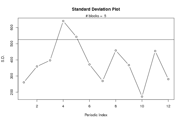
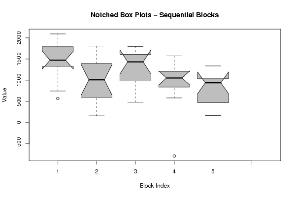
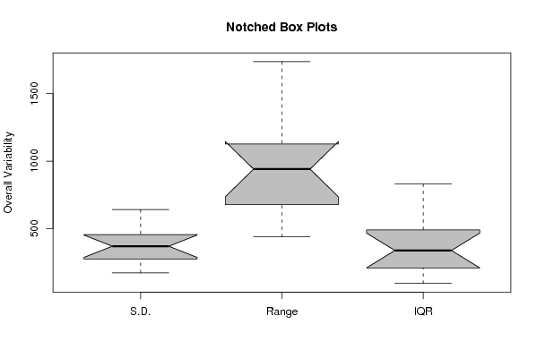
| Title produced by software | Standard Deviation Plot | ||||||||||||||||||||
| Date of computation | Sun, 15 Nov 2009 07:21:22 -0700 | ||||||||||||||||||||
| Cite this page as follows | Statistical Computations at FreeStatistics.org, Office for Research Development and Education, URL https://freestatistics.org/blog/index.php?v=date/2009/Nov/15/t1258294950fnvnempnyycbwmr.htm/, Retrieved Wed, 02 Jul 2025 15:52:50 +0000 | ||||||||||||||||||||
| Statistical Computations at FreeStatistics.org, Office for Research Development and Education, URL https://freestatistics.org/blog/index.php?pk=57292, Retrieved Wed, 02 Jul 2025 15:52:50 +0000 | |||||||||||||||||||||
| QR Codes: | |||||||||||||||||||||
|
| |||||||||||||||||||||
| Original text written by user: | |||||||||||||||||||||
| IsPrivate? | No (this computation is public) | ||||||||||||||||||||
| User-defined keywords | |||||||||||||||||||||
| Estimated Impact | 314 | ||||||||||||||||||||
Tree of Dependent Computations | |||||||||||||||||||||
| Family? (F = Feedback message, R = changed R code, M = changed R Module, P = changed Parameters, D = changed Data) | |||||||||||||||||||||
| - [Standard Deviation Plot] [3/11/2009] [2009-11-02 22:09:58] [b98453cac15ba1066b407e146608df68] - PD [Standard Deviation Plot] [Workshop 6] [2009-11-09 11:15:14] [3e19a07d230ba260a720e0e03e0f40f2] - D [Standard Deviation Plot] [WS6] [2009-11-15 14:21:22] [48076ccf082563ab8a2c81e57fdb5364] [Current] | |||||||||||||||||||||
| Feedback Forum | |||||||||||||||||||||
Post a new message | |||||||||||||||||||||
Dataset | |||||||||||||||||||||
| Dataseries X: | |||||||||||||||||||||
745,52 1962,64 2092,88 2034,73 568,28 1482,67 1282,26 1534,16 1621,42 1465,32 1373,15 1386,28 756,10 1359,02 1600,69 1299,97 161,31 622,74 552,60 570,36 806,43 1212,24 1806,54 1433,47 543,97 1453,00 1795,89 1608,99 484,29 1541,01 1094,14 1412,93 1612,35 1309,29 1626,17 874,45 794,25 1416,23 1575,25 1255,68 -787,86 1038,52 934,94 581,78 1069,98 1104,77 1152,28 880,48 169,49 953,93 1009,01 297,91 259,98 1164,90 924,60 840,77 1042,04 1026,08 637,53 1338,82 | |||||||||||||||||||||
Tables (Output of Computation) | |||||||||||||||||||||
| |||||||||||||||||||||
Figures (Output of Computation) | |||||||||||||||||||||
Input Parameters & R Code | |||||||||||||||||||||
| Parameters (Session): | |||||||||||||||||||||
| par1 = 12 ; | |||||||||||||||||||||
| Parameters (R input): | |||||||||||||||||||||
| par1 = 12 ; | |||||||||||||||||||||
| R code (references can be found in the software module): | |||||||||||||||||||||
par1 <- as.numeric(par1) | |||||||||||||||||||||