Free Statistics
of Irreproducible Research!
Description of Statistical Computation | |||||||||||||||||||||
|---|---|---|---|---|---|---|---|---|---|---|---|---|---|---|---|---|---|---|---|---|---|
| Author's title | |||||||||||||||||||||
| Author | *The author of this computation has been verified* | ||||||||||||||||||||
| R Software Module | rwasp_sdplot.wasp | ||||||||||||||||||||
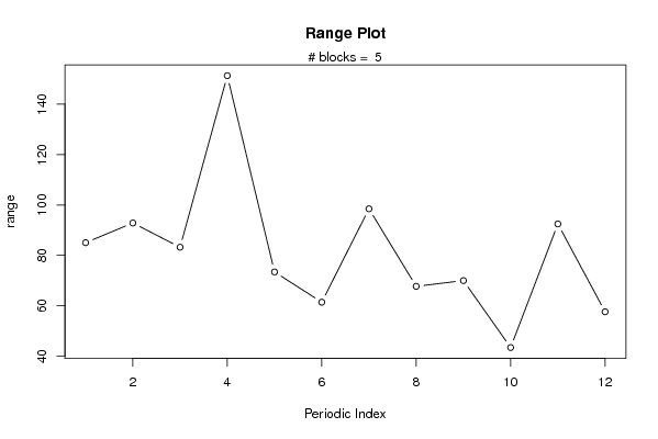
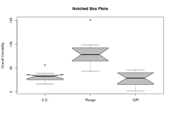
| Title produced by software | Standard Deviation Plot | ||||||||||||||||||||
| Date of computation | Fri, 13 Nov 2009 12:42:34 -0700 | ||||||||||||||||||||
| Cite this page as follows | Statistical Computations at FreeStatistics.org, Office for Research Development and Education, URL https://freestatistics.org/blog/index.php?v=date/2009/Nov/13/t12581413725dosh0cjq79m829.htm/, Retrieved Mon, 18 May 2026 09:49:22 +0000 | ||||||||||||||||||||
| Statistical Computations at FreeStatistics.org, Office for Research Development and Education, URL https://freestatistics.org/blog/index.php?pk=57054, Retrieved Mon, 18 May 2026 09:49:22 +0000 | |||||||||||||||||||||
| QR Codes: | |||||||||||||||||||||
|
| |||||||||||||||||||||
| Original text written by user: | |||||||||||||||||||||
| IsPrivate? | No (this computation is public) | ||||||||||||||||||||
| User-defined keywords | |||||||||||||||||||||
| Estimated Impact | 363 | ||||||||||||||||||||
Tree of Dependent Computations | |||||||||||||||||||||
| Family? (F = Feedback message, R = changed R code, M = changed R Module, P = changed Parameters, D = changed Data) | |||||||||||||||||||||
| - [Standard Deviation Plot] [3/11/2009] [2009-11-02 22:09:58] [b98453cac15ba1066b407e146608df68] - R D [Standard Deviation Plot] [] [2009-11-11 15:55:48] [74be16979710d4c4e7c6647856088456] - PD [Standard Deviation Plot] [] [2009-11-13 19:42:34] [f066b5fba39549422fd1c7a1f2ce0075] [Current] | |||||||||||||||||||||
| Feedback Forum | |||||||||||||||||||||
Post a new message | |||||||||||||||||||||
Dataset | |||||||||||||||||||||
| Dataseries X: | |||||||||||||||||||||
153,24 184,48 191,81 168,19 163,81 190,57 163,81 129,62 173,90 198,76 135,52 179,81 137,05 142,57 187,52 220,48 208,76 210,19 232,57 173,81 218,86 226,76 196,67 237,43 173,14 207,62 234,67 204,10 230,76 210,19 194,76 172,10 221,90 225,24 228,00 198,76 199,05 235,43 270,76 234,10 237,24 239,43 239,24 197,33 217,43 242,19 207,52 232,76 222,10 202,48 228,10 319,52 236,95 252,00 262,29 172,10 243,90 235,62 216,95 236,29 | |||||||||||||||||||||
Tables (Output of Computation) | |||||||||||||||||||||
| |||||||||||||||||||||
Figures (Output of Computation) | |||||||||||||||||||||
Input Parameters & R Code | |||||||||||||||||||||
| Parameters (Session): | |||||||||||||||||||||
| par1 = 12 ; | |||||||||||||||||||||
| Parameters (R input): | |||||||||||||||||||||
| par1 = 12 ; | |||||||||||||||||||||
| R code (references can be found in the software module): | |||||||||||||||||||||
par1 <- as.numeric(par1) | |||||||||||||||||||||