Free Statistics
of Irreproducible Research!
Description of Statistical Computation | |||||||||||||||||||||||||||||||||||||||||||||||||||||
|---|---|---|---|---|---|---|---|---|---|---|---|---|---|---|---|---|---|---|---|---|---|---|---|---|---|---|---|---|---|---|---|---|---|---|---|---|---|---|---|---|---|---|---|---|---|---|---|---|---|---|---|---|---|
| Author's title | |||||||||||||||||||||||||||||||||||||||||||||||||||||
| Author | *Unverified author* | ||||||||||||||||||||||||||||||||||||||||||||||||||||
| R Software Module | rwasp_edauni.wasp | ||||||||||||||||||||||||||||||||||||||||||||||||||||
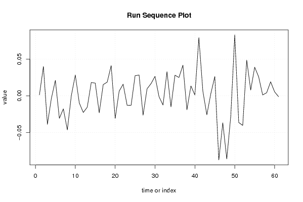
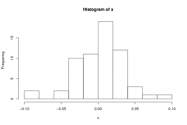
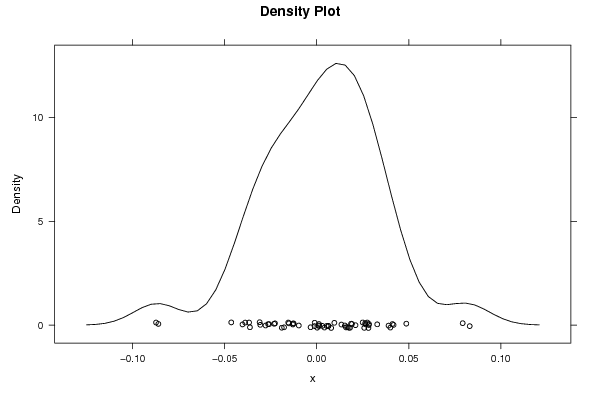
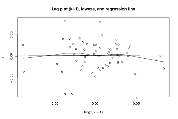
| Title produced by software | Univariate Explorative Data Analysis | ||||||||||||||||||||||||||||||||||||||||||||||||||||
| Date of computation | Thu, 31 Dec 2009 04:25:34 -0700 | ||||||||||||||||||||||||||||||||||||||||||||||||||||
| Cite this page as follows | Statistical Computations at FreeStatistics.org, Office for Research Development and Education, URL https://freestatistics.org/blog/index.php?v=date/2009/Dec/31/t1262258788y2c47x4y66f6u5x.htm/, Retrieved Sun, 06 Jul 2025 17:29:12 +0000 | ||||||||||||||||||||||||||||||||||||||||||||||||||||
| Statistical Computations at FreeStatistics.org, Office for Research Development and Education, URL https://freestatistics.org/blog/index.php?pk=71450, Retrieved Sun, 06 Jul 2025 17:29:12 +0000 | |||||||||||||||||||||||||||||||||||||||||||||||||||||
| QR Codes: | |||||||||||||||||||||||||||||||||||||||||||||||||||||
|
| |||||||||||||||||||||||||||||||||||||||||||||||||||||
| Original text written by user: | |||||||||||||||||||||||||||||||||||||||||||||||||||||
| IsPrivate? | No (this computation is public) | ||||||||||||||||||||||||||||||||||||||||||||||||||||
| User-defined keywords | |||||||||||||||||||||||||||||||||||||||||||||||||||||
| Estimated Impact | 253 | ||||||||||||||||||||||||||||||||||||||||||||||||||||
Tree of Dependent Computations | |||||||||||||||||||||||||||||||||||||||||||||||||||||
| Family? (F = Feedback message, R = changed R code, M = changed R Module, P = changed Parameters, D = changed Data) | |||||||||||||||||||||||||||||||||||||||||||||||||||||
| - [Univariate Data Series] [data set] [2008-12-01 19:54:57] [b98453cac15ba1066b407e146608df68] - RMP [ARIMA Backward Selection] [] [2009-11-27 14:53:14] [b98453cac15ba1066b407e146608df68] - PD [ARIMA Backward Selection] [Workshop 9 - Arim...] [2009-12-03 16:04:59] [1646a2766cb8c4a6f9d3b2fffef409b3] - RMPD [Univariate Explorative Data Analysis] [Paper] [2009-12-31 11:25:34] [3ebad5d90a5c8606f133189c73066208] [Current] - PD [Univariate Explorative Data Analysis] [Paper Run an seq ...] [2010-12-11 15:05:44] [6e6854a111a7f2438dd668bfaa6f3aa0] - RMPD [ARIMA Forecasting] [Paper Arima forecast] [2010-12-11 15:15:10] [6e6854a111a7f2438dd668bfaa6f3aa0] - RMPD [Multiple Regression] [Paper multi regre...] [2010-12-11 16:45:31] [6e6854a111a7f2438dd668bfaa6f3aa0] | |||||||||||||||||||||||||||||||||||||||||||||||||||||
| Feedback Forum | |||||||||||||||||||||||||||||||||||||||||||||||||||||
Post a new message | |||||||||||||||||||||||||||||||||||||||||||||||||||||
Dataset | |||||||||||||||||||||||||||||||||||||||||||||||||||||
| Dataseries X: | |||||||||||||||||||||||||||||||||||||||||||||||||||||
0.00129909929391305 0.0399953455650052 -0.0388246377373741 -0.00331410653299091 0.0210839113108800 -0.0306161034410643 -0.0177106810085845 -0.046387990142741 0.000293807560611557 0.0283994201318544 -0.0097276499256617 -0.0226399010542774 -0.0154224216079923 0.0180996287729906 0.0174136599175999 -0.0230868312646511 0.0152995239008014 0.0186909303105856 0.0411546583121751 -0.0309853409627296 0.00641105220624505 0.0159182504768269 -0.0129464581053229 -0.0128078454602796 0.0274724628079561 0.0283118917490450 -0.0263638289790966 0.00959383292935723 0.0166833770244468 0.0265094201387677 -0.00109417116631749 -0.0125243883301391 0.0328788388222352 -0.0150708239891775 0.0280916856622302 0.0249707612360408 0.0417384790369306 -0.0189545400438149 0.0134272541571829 0.00114937541706439 0.0792737906675707 0.00631274994392772 -0.0258498505131595 0.00309104687364825 0.0263272745307186 -0.0872423105882159 -0.0367158144235664 -0.0859756758601653 -0.027777298319539 0.0830853071279365 -0.0362488888752577 -0.0402967807676649 0.0486619532670178 0.00786966021276925 0.0390206657243493 0.0258356960136144 0.00122924684045933 0.00419954182511484 0.0191498676670216 0.00542117110649887 -0.00117174374524698 | |||||||||||||||||||||||||||||||||||||||||||||||||||||
Tables (Output of Computation) | |||||||||||||||||||||||||||||||||||||||||||||||||||||
| |||||||||||||||||||||||||||||||||||||||||||||||||||||
Figures (Output of Computation) | |||||||||||||||||||||||||||||||||||||||||||||||||||||
Input Parameters & R Code | |||||||||||||||||||||||||||||||||||||||||||||||||||||
| Parameters (Session): | |||||||||||||||||||||||||||||||||||||||||||||||||||||
| par1 = 0 ; par2 = 36 ; | |||||||||||||||||||||||||||||||||||||||||||||||||||||
| Parameters (R input): | |||||||||||||||||||||||||||||||||||||||||||||||||||||
| par1 = 0 ; par2 = 36 ; | |||||||||||||||||||||||||||||||||||||||||||||||||||||
| R code (references can be found in the software module): | |||||||||||||||||||||||||||||||||||||||||||||||||||||
par1 <- as.numeric(par1) | |||||||||||||||||||||||||||||||||||||||||||||||||||||