Free Statistics
of Irreproducible Research!
Description of Statistical Computation | |||||||||||||||||||||
|---|---|---|---|---|---|---|---|---|---|---|---|---|---|---|---|---|---|---|---|---|---|
| Author's title | |||||||||||||||||||||
| Author | *The author of this computation has been verified* | ||||||||||||||||||||
| R Software Module | rwasp_meanplot.wasp | ||||||||||||||||||||
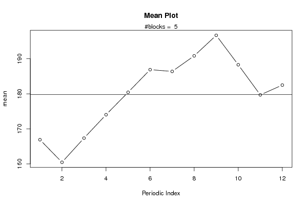
| Title produced by software | Mean Plot | ||||||||||||||||||||
| Date of computation | Wed, 09 Dec 2009 10:46:09 -0700 | ||||||||||||||||||||
| Cite this page as follows | Statistical Computations at FreeStatistics.org, Office for Research Development and Education, URL https://freestatistics.org/blog/index.php?v=date/2009/Dec/09/t12603811213tlacwwzdilnabv.htm/, Retrieved Thu, 21 May 2026 00:47:53 +0000 | ||||||||||||||||||||
| Statistical Computations at FreeStatistics.org, Office for Research Development and Education, URL https://freestatistics.org/blog/index.php?pk=65097, Retrieved Thu, 21 May 2026 00:47:53 +0000 | |||||||||||||||||||||
| QR Codes: | |||||||||||||||||||||
|
| |||||||||||||||||||||
| Original text written by user: | |||||||||||||||||||||
| IsPrivate? | No (this computation is public) | ||||||||||||||||||||
| User-defined keywords | |||||||||||||||||||||
| Estimated Impact | 416 | ||||||||||||||||||||
Tree of Dependent Computations | |||||||||||||||||||||
| Family? (F = Feedback message, R = changed R code, M = changed R Module, P = changed Parameters, D = changed Data) | |||||||||||||||||||||
| - [Mean Plot] [Mean Plot Graan] [2007-11-30 10:04:32] [ccd50806b5892327d2f6528fe41d0c23] - M D [Mean Plot] [paper mean plot] [2009-12-09 17:46:09] [51d49d3536f6a59f2486a67bf50b2759] [Current] - D [Mean Plot] [paper mean plot t...] [2009-12-10 16:25:05] [12f02da0296cb21dc23d82ae014a8b71] - [Mean Plot] [mean plot totaal] [2009-12-21 14:57:24] [03c44f58d7d4de05d4cfabfda8c46d2c] - R D [Mean Plot] [mean plot] [2009-12-24 16:18:37] [757146c69eaf0537be37c7b0c18216d8] - [Mean Plot] [paper mean plot] [2009-12-21 15:27:32] [03c44f58d7d4de05d4cfabfda8c46d2c] - R D [Mean Plot] [bijlage paper] [2009-12-24 16:27:01] [757146c69eaf0537be37c7b0c18216d8] | |||||||||||||||||||||
| Feedback Forum | |||||||||||||||||||||
Post a new message | |||||||||||||||||||||
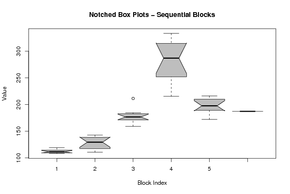
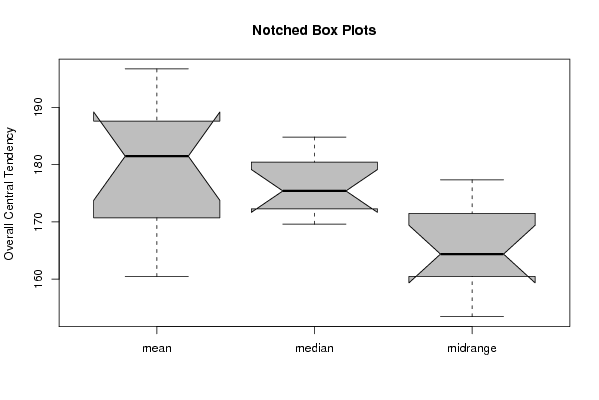
Dataset | |||||||||||||||||||||
| Dataseries X: | |||||||||||||||||||||
108,2 108,8 110,2 109,5 109,5 116 111,2 112,1 114 119,1 114,1 115,1 115,4 110,8 116 119,2 126,5 127,8 131,3 140,3 137,3 143 134,5 139,9 159,3 170,4 175 175,8 180,9 180,3 169,6 172,3 184,8 177,7 184,6 211,4 215,3 215,9 244,7 259,3 289 310,9 321 315,1 333,2 314,1 284,7 273,9 216 196,4 190,9 206,4 196,3 199,5 198,9 214,4 214,2 187,6 180,6 172,2 187,2 | |||||||||||||||||||||
Tables (Output of Computation) | |||||||||||||||||||||
| |||||||||||||||||||||
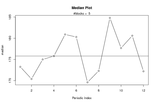
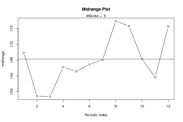
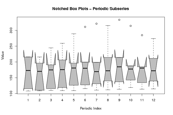
Figures (Output of Computation) | |||||||||||||||||||||
Input Parameters & R Code | |||||||||||||||||||||
| Parameters (Session): | |||||||||||||||||||||
| par1 = 12 ; | |||||||||||||||||||||
| Parameters (R input): | |||||||||||||||||||||
| par1 = 12 ; | |||||||||||||||||||||
| R code (references can be found in the software module): | |||||||||||||||||||||
par1 <- as.numeric(par1) | |||||||||||||||||||||