Free Statistics
of Irreproducible Research!
Description of Statistical Computation | |||||||||||||||||||||||||||||||||||||||||||||||||||||||||||||||||||||||||||||||||||||||||||||||||||||||||||||||||||||||||||||||||
|---|---|---|---|---|---|---|---|---|---|---|---|---|---|---|---|---|---|---|---|---|---|---|---|---|---|---|---|---|---|---|---|---|---|---|---|---|---|---|---|---|---|---|---|---|---|---|---|---|---|---|---|---|---|---|---|---|---|---|---|---|---|---|---|---|---|---|---|---|---|---|---|---|---|---|---|---|---|---|---|---|---|---|---|---|---|---|---|---|---|---|---|---|---|---|---|---|---|---|---|---|---|---|---|---|---|---|---|---|---|---|---|---|---|---|---|---|---|---|---|---|---|---|---|---|---|---|---|---|---|
| Author's title | |||||||||||||||||||||||||||||||||||||||||||||||||||||||||||||||||||||||||||||||||||||||||||||||||||||||||||||||||||||||||||||||||
| Author | *The author of this computation has been verified* | ||||||||||||||||||||||||||||||||||||||||||||||||||||||||||||||||||||||||||||||||||||||||||||||||||||||||||||||||||||||||||||||||
| R Software Module | rwasp_smp.wasp | ||||||||||||||||||||||||||||||||||||||||||||||||||||||||||||||||||||||||||||||||||||||||||||||||||||||||||||||||||||||||||||||||
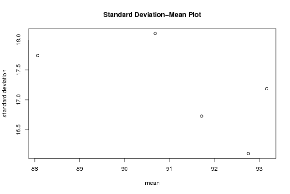
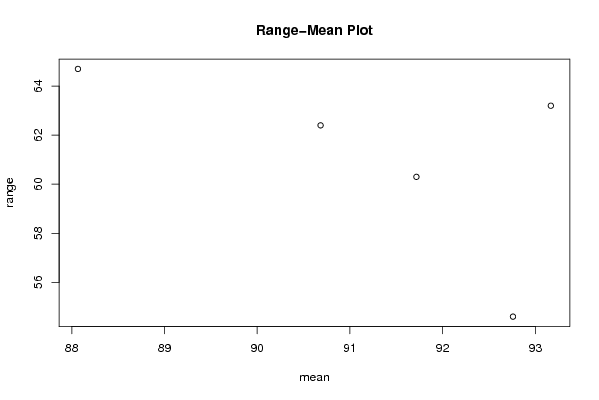
| Title produced by software | Standard Deviation-Mean Plot | ||||||||||||||||||||||||||||||||||||||||||||||||||||||||||||||||||||||||||||||||||||||||||||||||||||||||||||||||||||||||||||||||
| Date of computation | Sat, 29 Nov 2008 17:31:28 -0700 | ||||||||||||||||||||||||||||||||||||||||||||||||||||||||||||||||||||||||||||||||||||||||||||||||||||||||||||||||||||||||||||||||
| Cite this page as follows | Statistical Computations at FreeStatistics.org, Office for Research Development and Education, URL https://freestatistics.org/blog/index.php?v=date/2008/Nov/30/t1228005218xvnvg84xodvlket.htm/, Retrieved Wed, 05 Nov 2025 17:05:13 +0000 | ||||||||||||||||||||||||||||||||||||||||||||||||||||||||||||||||||||||||||||||||||||||||||||||||||||||||||||||||||||||||||||||||
| Statistical Computations at FreeStatistics.org, Office for Research Development and Education, URL https://freestatistics.org/blog/index.php?pk=26395, Retrieved Wed, 05 Nov 2025 17:05:13 +0000 | |||||||||||||||||||||||||||||||||||||||||||||||||||||||||||||||||||||||||||||||||||||||||||||||||||||||||||||||||||||||||||||||||
| QR Codes: | |||||||||||||||||||||||||||||||||||||||||||||||||||||||||||||||||||||||||||||||||||||||||||||||||||||||||||||||||||||||||||||||||
|
| |||||||||||||||||||||||||||||||||||||||||||||||||||||||||||||||||||||||||||||||||||||||||||||||||||||||||||||||||||||||||||||||||
| Original text written by user: | |||||||||||||||||||||||||||||||||||||||||||||||||||||||||||||||||||||||||||||||||||||||||||||||||||||||||||||||||||||||||||||||||
| IsPrivate? | No (this computation is public) | ||||||||||||||||||||||||||||||||||||||||||||||||||||||||||||||||||||||||||||||||||||||||||||||||||||||||||||||||||||||||||||||||
| User-defined keywords | |||||||||||||||||||||||||||||||||||||||||||||||||||||||||||||||||||||||||||||||||||||||||||||||||||||||||||||||||||||||||||||||||
| Estimated Impact | 428 | ||||||||||||||||||||||||||||||||||||||||||||||||||||||||||||||||||||||||||||||||||||||||||||||||||||||||||||||||||||||||||||||||
Tree of Dependent Computations | |||||||||||||||||||||||||||||||||||||||||||||||||||||||||||||||||||||||||||||||||||||||||||||||||||||||||||||||||||||||||||||||||
| Family? (F = Feedback message, R = changed R code, M = changed R Module, P = changed Parameters, D = changed Data) | |||||||||||||||||||||||||||||||||||||||||||||||||||||||||||||||||||||||||||||||||||||||||||||||||||||||||||||||||||||||||||||||||
| F [Univariate Data Series] [Airline data] [2007-10-18 09:58:47] [42daae401fd3def69a25014f2252b4c2] F RMPD [Standard Deviation-Mean Plot] [Q5 Standard DMP] [2008-11-29 16:26:32] [aa5573c1db401b164e448aef050955a1] - PD [Standard Deviation-Mean Plot] [Q8 SDMN bouwprod] [2008-11-30 00:14:02] [aa5573c1db401b164e448aef050955a1] - [Standard Deviation-Mean Plot] [Q8 SDMN bouwprod] [2008-11-30 00:31:28] [8a1195ff8db4df756ce44b463a631c76] [Current] - P [Standard Deviation-Mean Plot] [Standard Deviatio...] [2008-12-12 12:06:26] [aa5573c1db401b164e448aef050955a1] - P [Standard Deviation-Mean Plot] [Standard Deviatio...] [2008-12-12 12:06:26] [aa5573c1db401b164e448aef050955a1] - P [Standard Deviation-Mean Plot] [Standard Deviatio...] [2008-12-12 12:06:26] [aa5573c1db401b164e448aef050955a1] - RMP [Box-Cox Normality Plot] [Box Cox Normality...] [2008-12-12 12:35:24] [aa5573c1db401b164e448aef050955a1] - RM [Variance Reduction Matrix] [VRM Bouwproductie] [2008-12-12 13:22:47] [aa5573c1db401b164e448aef050955a1] - RMP [(Partial) Autocorrelation Function] [ACF bouwproductie...] [2008-12-12 13:31:29] [aa5573c1db401b164e448aef050955a1] - P [(Partial) Autocorrelation Function] [ACF bouwproductie...] [2008-12-12 13:45:52] [aa5573c1db401b164e448aef050955a1] - P [(Partial) Autocorrelation Function] [ACF bouwproductie...] [2008-12-12 13:59:06] [aa5573c1db401b164e448aef050955a1] - RM [Spectral Analysis] [Spectral Analysis...] [2008-12-12 14:26:07] [aa5573c1db401b164e448aef050955a1] - RM [Spectral Analysis] [Spectral Analysis...] [2008-12-12 14:42:38] [aa5573c1db401b164e448aef050955a1] - D [Standard Deviation-Mean Plot] [SDMP Totale Produ...] [2008-12-12 15:57:50] [aa5573c1db401b164e448aef050955a1] - RM [Variance Reduction Matrix] [VRM Totale Productie] [2008-12-12 16:00:44] [aa5573c1db401b164e448aef050955a1] - RMPD [Cross Correlation Function] [CCF Bouwproductie...] [2008-12-12 16:06:05] [aa5573c1db401b164e448aef050955a1] - P [Cross Correlation Function] [CCF Bouwproductie...] [2008-12-12 16:12:34] [aa5573c1db401b164e448aef050955a1] | |||||||||||||||||||||||||||||||||||||||||||||||||||||||||||||||||||||||||||||||||||||||||||||||||||||||||||||||||||||||||||||||||
| Feedback Forum | |||||||||||||||||||||||||||||||||||||||||||||||||||||||||||||||||||||||||||||||||||||||||||||||||||||||||||||||||||||||||||||||||
Post a new message | |||||||||||||||||||||||||||||||||||||||||||||||||||||||||||||||||||||||||||||||||||||||||||||||||||||||||||||||||||||||||||||||||
Dataset | |||||||||||||||||||||||||||||||||||||||||||||||||||||||||||||||||||||||||||||||||||||||||||||||||||||||||||||||||||||||||||||||||
| Dataseries X: | |||||||||||||||||||||||||||||||||||||||||||||||||||||||||||||||||||||||||||||||||||||||||||||||||||||||||||||||||||||||||||||||||
82.7 88.9 105.9 100.8 94 105 58.5 87.6 113.1 112.5 89.6 74.5 82.7 90.1 109.4 96 89.2 109.1 49.1 92.9 107.7 103.5 91.1 79.8 71.9 82.9 90.1 100.7 90.7 108.8 44.1 93.6 107.4 96.5 93.6 76.5 76.7 84 103.3 88.5 99 105.9 44.7 94 107.1 104.8 102.5 77.7 85.2 91.3 106.5 92.4 97.5 107 51.1 98.6 102.2 114.3 99.4 72.5 92.3 99.4 85.9 109.4 97.6 | |||||||||||||||||||||||||||||||||||||||||||||||||||||||||||||||||||||||||||||||||||||||||||||||||||||||||||||||||||||||||||||||||
Tables (Output of Computation) | |||||||||||||||||||||||||||||||||||||||||||||||||||||||||||||||||||||||||||||||||||||||||||||||||||||||||||||||||||||||||||||||||
| |||||||||||||||||||||||||||||||||||||||||||||||||||||||||||||||||||||||||||||||||||||||||||||||||||||||||||||||||||||||||||||||||
Figures (Output of Computation) | |||||||||||||||||||||||||||||||||||||||||||||||||||||||||||||||||||||||||||||||||||||||||||||||||||||||||||||||||||||||||||||||||
Input Parameters & R Code | |||||||||||||||||||||||||||||||||||||||||||||||||||||||||||||||||||||||||||||||||||||||||||||||||||||||||||||||||||||||||||||||||
| Parameters (Session): | |||||||||||||||||||||||||||||||||||||||||||||||||||||||||||||||||||||||||||||||||||||||||||||||||||||||||||||||||||||||||||||||||
| par1 = 1 ; par2 = 0 ; par3 = 1 ; par4 = 1 ; par5 = 1 ; par6 = 0 ; par7 = 1 ; | |||||||||||||||||||||||||||||||||||||||||||||||||||||||||||||||||||||||||||||||||||||||||||||||||||||||||||||||||||||||||||||||||
| Parameters (R input): | |||||||||||||||||||||||||||||||||||||||||||||||||||||||||||||||||||||||||||||||||||||||||||||||||||||||||||||||||||||||||||||||||
| par1 = 12 ; | |||||||||||||||||||||||||||||||||||||||||||||||||||||||||||||||||||||||||||||||||||||||||||||||||||||||||||||||||||||||||||||||||
| R code (references can be found in the software module): | |||||||||||||||||||||||||||||||||||||||||||||||||||||||||||||||||||||||||||||||||||||||||||||||||||||||||||||||||||||||||||||||||
par1 <- as.numeric(par1) | |||||||||||||||||||||||||||||||||||||||||||||||||||||||||||||||||||||||||||||||||||||||||||||||||||||||||||||||||||||||||||||||||