Free Statistics
of Irreproducible Research!
Description of Statistical Computation | |||||||||||||||||||||||||||||||||||||
|---|---|---|---|---|---|---|---|---|---|---|---|---|---|---|---|---|---|---|---|---|---|---|---|---|---|---|---|---|---|---|---|---|---|---|---|---|---|
| Author's title | |||||||||||||||||||||||||||||||||||||
| Author | *The author of this computation has been verified* | ||||||||||||||||||||||||||||||||||||
| R Software Module | rwasp_boxcoxnorm.wasp | ||||||||||||||||||||||||||||||||||||
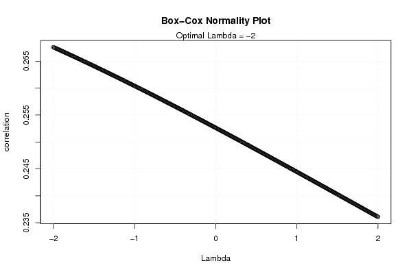
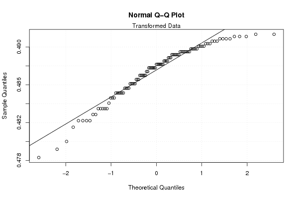
| Title produced by software | Box-Cox Normality Plot | ||||||||||||||||||||||||||||||||||||
| Date of computation | Wed, 12 Nov 2008 05:32:59 -0700 | ||||||||||||||||||||||||||||||||||||
| Cite this page as follows | Statistical Computations at FreeStatistics.org, Office for Research Development and Education, URL https://freestatistics.org/blog/index.php?v=date/2008/Nov/12/t12264932480uwzlyq824o1gwp.htm/, Retrieved Fri, 04 Jul 2025 09:57:25 +0000 | ||||||||||||||||||||||||||||||||||||
| Statistical Computations at FreeStatistics.org, Office for Research Development and Education, URL https://freestatistics.org/blog/index.php?pk=24154, Retrieved Fri, 04 Jul 2025 09:57:25 +0000 | |||||||||||||||||||||||||||||||||||||
| QR Codes: | |||||||||||||||||||||||||||||||||||||
|
| |||||||||||||||||||||||||||||||||||||
| Original text written by user: | |||||||||||||||||||||||||||||||||||||
| IsPrivate? | No (this computation is public) | ||||||||||||||||||||||||||||||||||||
| User-defined keywords | |||||||||||||||||||||||||||||||||||||
| Estimated Impact | 261 | ||||||||||||||||||||||||||||||||||||
Tree of Dependent Computations | |||||||||||||||||||||||||||||||||||||
| Family? (F = Feedback message, R = changed R code, M = changed R Module, P = changed Parameters, D = changed Data) | |||||||||||||||||||||||||||||||||||||
| F [Box-Cox Normality Plot] [Box-cox normality...] [2008-11-12 12:32:59] [a16dfd7e948381d8b6391003c5d09447] [Current] F D [Box-Cox Normality Plot] [opdracht3_Q4] [2008-11-12 15:45:57] [3f66c6f083b1153972739491b89fa2dd] | |||||||||||||||||||||||||||||||||||||
| Feedback Forum | |||||||||||||||||||||||||||||||||||||
Post a new message | |||||||||||||||||||||||||||||||||||||
Dataset | |||||||||||||||||||||||||||||||||||||
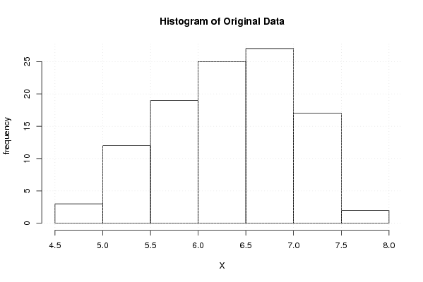
| Dataseries X: | |||||||||||||||||||||||||||||||||||||
6,6 6,4 6 5,8 5,5 5,4 5,4 5,6 5,5 5,8 5,8 5,7 5,5 5,3 5,2 5,3 5,3 5 4,8 4,9 5,3 6 6,2 6,4 6,4 6,4 6,2 6,1 6 5,9 6,2 6,2 6,4 6,8 6,9 7 7 6,9 6,7 6,6 6,5 6,4 6,5 6,5 6,6 6,7 6,8 7,2 7,6 7,6 7,3 6,4 6,1 6,3 7,1 7,5 7,4 7,1 6,8 6,9 7,2 7,4 7,3 6,9 6,9 6,8 7,1 7,2 7,1 7 6,9 7 7,4 7,5 7,5 7,4 7,3 7 6,7 6,5 6,5 6,5 6,6 6,8 6,9 6,9 6,8 6,8 6,5 6,1 6 5,9 5,8 5,9 5,9 6,2 6,3 6,2 6 5,8 5,5 5,5 5,7 5,8 5,7 | |||||||||||||||||||||||||||||||||||||
Tables (Output of Computation) | |||||||||||||||||||||||||||||||||||||
| |||||||||||||||||||||||||||||||||||||
Figures (Output of Computation) | |||||||||||||||||||||||||||||||||||||
Input Parameters & R Code | |||||||||||||||||||||||||||||||||||||
| Parameters (Session): | |||||||||||||||||||||||||||||||||||||
| Parameters (R input): | |||||||||||||||||||||||||||||||||||||
| R code (references can be found in the software module): | |||||||||||||||||||||||||||||||||||||
n <- length(x) | |||||||||||||||||||||||||||||||||||||