Free Statistics
of Irreproducible Research!
Description of Statistical Computation | |||||||||||||||||||||||||||||||||||||
|---|---|---|---|---|---|---|---|---|---|---|---|---|---|---|---|---|---|---|---|---|---|---|---|---|---|---|---|---|---|---|---|---|---|---|---|---|---|
| Author's title | |||||||||||||||||||||||||||||||||||||
| Author | *The author of this computation has been verified* | ||||||||||||||||||||||||||||||||||||
| R Software Module | rwasp_boxcoxnorm.wasp | ||||||||||||||||||||||||||||||||||||
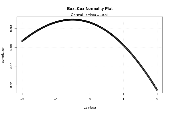
| Title produced by software | Box-Cox Normality Plot | ||||||||||||||||||||||||||||||||||||
| Date of computation | Tue, 11 Nov 2008 15:29:05 -0700 | ||||||||||||||||||||||||||||||||||||
| Cite this page as follows | Statistical Computations at FreeStatistics.org, Office for Research Development and Education, URL https://freestatistics.org/blog/index.php?v=date/2008/Nov/11/t1226442627grpa96cki5jomkn.htm/, Retrieved Sat, 16 May 2026 03:08:56 +0000 | ||||||||||||||||||||||||||||||||||||
| Statistical Computations at FreeStatistics.org, Office for Research Development and Education, URL https://freestatistics.org/blog/index.php?pk=24004, Retrieved Sat, 16 May 2026 03:08:56 +0000 | |||||||||||||||||||||||||||||||||||||
| QR Codes: | |||||||||||||||||||||||||||||||||||||
|
| |||||||||||||||||||||||||||||||||||||
| Original text written by user: | |||||||||||||||||||||||||||||||||||||
| IsPrivate? | No (this computation is public) | ||||||||||||||||||||||||||||||||||||
| User-defined keywords | |||||||||||||||||||||||||||||||||||||
| Estimated Impact | 458 | ||||||||||||||||||||||||||||||||||||
Tree of Dependent Computations | |||||||||||||||||||||||||||||||||||||
| Family? (F = Feedback message, R = changed R code, M = changed R Module, P = changed Parameters, D = changed Data) | |||||||||||||||||||||||||||||||||||||
| F [Box-Cox Normality Plot] [Various EDA topic...] [2008-11-11 22:29:05] [382e90e66f02be5ed86892bdc1574692] [Current] F RM D [Partial Correlation] [Various EDA topic...] [2008-11-11 22:49:47] [d32f94eec6fe2d8c421bd223368a5ced] F RMP [Trivariate Scatterplots] [Various EDA topic...] [2008-11-11 23:06:10] [d32f94eec6fe2d8c421bd223368a5ced] F D [Box-Cox Normality Plot] [Q4] [2008-11-12 13:48:50] [74be16979710d4c4e7c6647856088456] F D [Box-Cox Normality Plot] [] [2008-11-12 13:51:20] [8d2ae74f923b31b35e9e42977c3c4399] | |||||||||||||||||||||||||||||||||||||
| Feedback Forum | |||||||||||||||||||||||||||||||||||||
Post a new message | |||||||||||||||||||||||||||||||||||||
Dataset | |||||||||||||||||||||||||||||||||||||
| Dataseries X: | |||||||||||||||||||||||||||||||||||||
24,67 25,59 26,09 28,37 27,34 24,46 27,46 30,23 32,33 29,87 24,87 25,48 27,28 28,24 29,58 26,95 29,08 28,76 29,59 30,7 30,52 32,67 33,19 37,13 35,54 37,75 41,84 42,94 49,14 44,61 40,22 44,23 45,85 53,38 53,26 51,8 55,3 57,81 63,96 63,77 59,15 56,12 57,42 63,52 61,71 63,01 68,18 72,03 69,75 74,41 74,33 64,24 60,03 59,44 62,5 55,04 58,34 61,92 67,65 67,68 | |||||||||||||||||||||||||||||||||||||
Tables (Output of Computation) | |||||||||||||||||||||||||||||||||||||
| |||||||||||||||||||||||||||||||||||||
Figures (Output of Computation) | |||||||||||||||||||||||||||||||||||||
Input Parameters & R Code | |||||||||||||||||||||||||||||||||||||
| Parameters (Session): | |||||||||||||||||||||||||||||||||||||
| Parameters (R input): | |||||||||||||||||||||||||||||||||||||
| R code (references can be found in the software module): | |||||||||||||||||||||||||||||||||||||
n <- length(x) | |||||||||||||||||||||||||||||||||||||