Free Statistics
of Irreproducible Research!
Description of Statistical Computation | |||||||||||||||||||||
|---|---|---|---|---|---|---|---|---|---|---|---|---|---|---|---|---|---|---|---|---|---|
| Author's title | |||||||||||||||||||||
| Author | *The author of this computation has been verified* | ||||||||||||||||||||
| R Software Module | rwasp_cloud.wasp | ||||||||||||||||||||
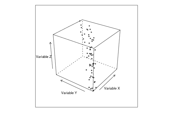
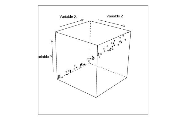
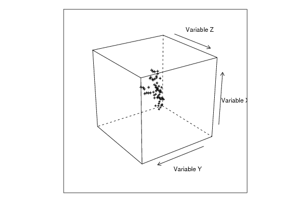
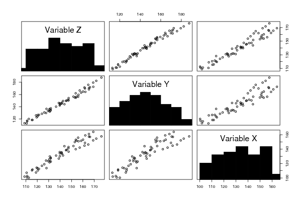
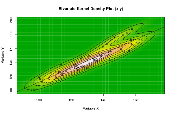
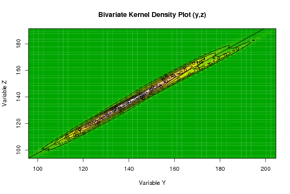
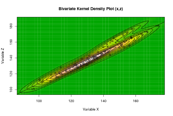
| Title produced by software | Trivariate Scatterplots | ||||||||||||||||||||
| Date of computation | Mon, 10 Nov 2008 05:27:32 -0700 | ||||||||||||||||||||
| Cite this page as follows | Statistical Computations at FreeStatistics.org, Office for Research Development and Education, URL https://freestatistics.org/blog/index.php?v=date/2008/Nov/10/t1226320106mhnrj902h3xahzx.htm/, Retrieved Thu, 01 Jan 2026 23:06:26 +0000 | ||||||||||||||||||||
| Statistical Computations at FreeStatistics.org, Office for Research Development and Education, URL https://freestatistics.org/blog/index.php?pk=22993, Retrieved Thu, 01 Jan 2026 23:06:26 +0000 | |||||||||||||||||||||
| QR Codes: | |||||||||||||||||||||
|
| |||||||||||||||||||||
| Original text written by user: | |||||||||||||||||||||
| IsPrivate? | No (this computation is public) | ||||||||||||||||||||
| User-defined keywords | |||||||||||||||||||||
| Estimated Impact | 464 | ||||||||||||||||||||
Tree of Dependent Computations | |||||||||||||||||||||
| Family? (F = Feedback message, R = changed R code, M = changed R Module, P = changed Parameters, D = changed Data) | |||||||||||||||||||||
| F [Trivariate Scatterplots] [Trivariate Scatte...] [2008-11-10 12:27:32] [e515c0250d6233b5d2604259ab52cebe] [Current] - RMPD [Testing Mean with known Variance - Critical Value] [Q1 Pork quality test] [2008-11-10 12:49:50] [5161246d1ccc1b670cc664d03050f084] F RMPD [Testing Mean with known Variance - Critical Value] [q1 pork quality test] [2008-11-10 12:51:44] [5161246d1ccc1b670cc664d03050f084] F RMPD [Testing Mean with known Variance - p-value] [Q2 pork quality test] [2008-11-10 12:58:58] [5161246d1ccc1b670cc664d03050f084] F RMPD [Testing Mean with known Variance - Type II Error] [Q3 pork qality test] [2008-11-10 13:08:48] [5161246d1ccc1b670cc664d03050f084] F RMPD [Testing Mean with known Variance - Sample Size] [q4 pork quality test] [2008-11-10 13:17:48] [5161246d1ccc1b670cc664d03050f084] F RMPD [Testing Population Mean with known Variance - Confidence Interval] [q5 pork quality test] [2008-11-10 13:23:22] [5161246d1ccc1b670cc664d03050f084] F RMPD [Testing Sample Mean with known Variance - Confidence Interval] [q6 pork quality test] [2008-11-10 13:30:42] [5161246d1ccc1b670cc664d03050f084] | |||||||||||||||||||||
| Feedback Forum | |||||||||||||||||||||
Post a new message | |||||||||||||||||||||
Dataset | |||||||||||||||||||||
| Dataseries X: | |||||||||||||||||||||
136.5 146.4 157.7 148.7 154.6 152.1 144.8 142.1 157 159.1 164 151.5 135.9 138.5 161 151.7 142.9 157.4 138.9 141 150.9 149.9 153 144.3 128.1 123.3 155.9 144.1 134.1 153.1 131 129.8 139.9 135.6 126.8 134.4 113.5 107.5 133.8 119 125.9 130.1 114.2 111.6 131.2 124.1 127.1 123.4 100.7 100.3 121.6 110.5 110.3 122.7 102.6 101.8 113.6 107.2 116.8 112.5 | |||||||||||||||||||||
| Dataseries Y: | |||||||||||||||||||||
154.2 175.8 187.6 169.9 182.3 179.4 171.5 166.6 171.8 164.3 172.6 163 142.2 149.7 168.4 156.5 150.4 170.6 150.1 151.5 159.5 155.2 154.8 156.5 134.2 135.9 156.4 144.2 143.7 164.8 140.2 132.2 162 145 146.3 145.5 124.4 126 146.8 130.8 133.6 145.7 122.8 118.5 149.5 129.9 134.8 133.3 117.2 120.2 136.4 118.5 126.7 137.5 116.3 113.3 136.6 112.9 128.6 126.8 | |||||||||||||||||||||
| Dataseries Z: | |||||||||||||||||||||
147.5 164.7 176.2 161.8 171.7 169 161.4 157.2 166.2 162.1 169.1 158.4 139.7 145.2 165.3 154.4 147.4 165.3 145.7 147.2 156.1 152.9 153.8 151.7 131.8 131 155.8 143.8 139.8 160.1 136.5 131 153.7 141.3 138.9 141.2 120.3 118.9 141.7 126.2 130.6 139.8 119.5 115.8 142.6 127.7 131.8 129.5 111.1 112.6 130.8 115.4 120.5 131.9 111.2 108.9 128.1 110.7 124.1 121.5 | |||||||||||||||||||||
Tables (Output of Computation) | |||||||||||||||||||||
| |||||||||||||||||||||
Figures (Output of Computation) | |||||||||||||||||||||
Input Parameters & R Code | |||||||||||||||||||||
| Parameters (Session): | |||||||||||||||||||||
| par1 = 50 ; par2 = 50 ; par3 = Y ; par4 = Y ; par5 = Variable X ; par6 = Variable Y ; par7 = Variable Z ; | |||||||||||||||||||||
| Parameters (R input): | |||||||||||||||||||||
| par1 = 50 ; par2 = 50 ; par3 = Y ; par4 = Y ; par5 = Variable X ; par6 = Variable Y ; par7 = Variable Z ; | |||||||||||||||||||||
| R code (references can be found in the software module): | |||||||||||||||||||||
x <- array(x,dim=c(length(x),1)) | |||||||||||||||||||||