Free Statistics
of Irreproducible Research!
Description of Statistical Computation | |||||||||||||||||||||||||||||||
|---|---|---|---|---|---|---|---|---|---|---|---|---|---|---|---|---|---|---|---|---|---|---|---|---|---|---|---|---|---|---|---|
| Author's title | |||||||||||||||||||||||||||||||
| Author | *The author of this computation has been verified* | ||||||||||||||||||||||||||||||
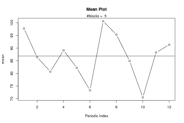
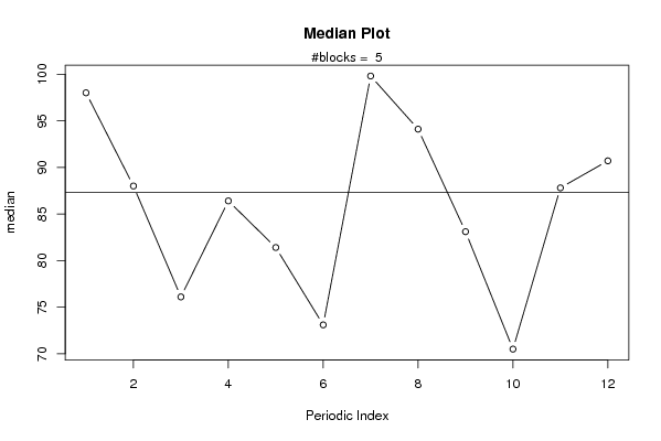
| R Software Module | rwasp_meanplot.wasp | ||||||||||||||||||||||||||||||
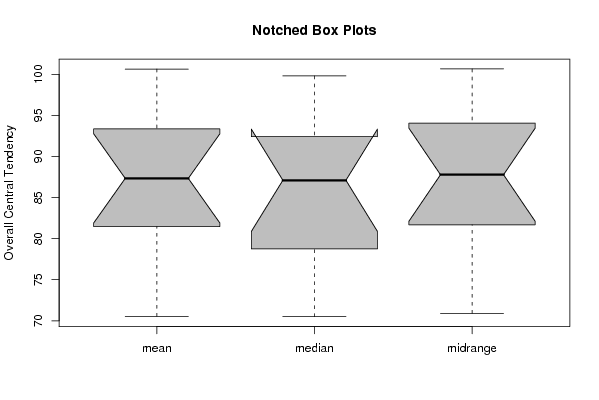
| Title produced by software | Mean Plot | ||||||||||||||||||||||||||||||
| Date of computation | Thu, 06 Nov 2008 09:32:30 -0700 | ||||||||||||||||||||||||||||||
| Cite this page as follows | Statistical Computations at FreeStatistics.org, Office for Research Development and Education, URL https://freestatistics.org/blog/index.php?v=date/2008/Nov/06/t1225989278w3uieksmmevl50g.htm/, Retrieved Sat, 05 Jul 2025 17:05:29 +0000 | ||||||||||||||||||||||||||||||
| Statistical Computations at FreeStatistics.org, Office for Research Development and Education, URL https://freestatistics.org/blog/index.php?pk=22317, Retrieved Sat, 05 Jul 2025 17:05:29 +0000 | |||||||||||||||||||||||||||||||
| QR Codes: | |||||||||||||||||||||||||||||||
|
| |||||||||||||||||||||||||||||||
| Original text written by user: | |||||||||||||||||||||||||||||||
| IsPrivate? | No (this computation is public) | ||||||||||||||||||||||||||||||
| User-defined keywords | |||||||||||||||||||||||||||||||
| Estimated Impact | 249 | ||||||||||||||||||||||||||||||
Tree of Dependent Computations | |||||||||||||||||||||||||||||||
| Family? (F = Feedback message, R = changed R code, M = changed R Module, P = changed Parameters, D = changed Data) | |||||||||||||||||||||||||||||||
| F [Mean Plot] [Mean Plot] [2008-11-06 16:32:30] [96839c4b6d4e03ef3851369c676780bf] [Current] - D [Mean Plot] [Mean Plot] [2008-12-22 08:12:49] [1a98f534d827b920a5783bf87d2d3cce] - RM D [Variance Reduction Matrix] [Variance Reductio...] [2008-12-22 09:53:55] [1a98f534d827b920a5783bf87d2d3cce] - RM D [Standard Deviation-Mean Plot] [Standard Deviatio...] [2008-12-22 11:03:46] [1a98f534d827b920a5783bf87d2d3cce] - RMPD [(Partial) Autocorrelation Function] [acf] [2008-12-22 12:36:13] [1a98f534d827b920a5783bf87d2d3cce] - RMPD [(Partial) Autocorrelation Function] [acf] [2008-12-22 12:41:23] [1a98f534d827b920a5783bf87d2d3cce] - RMPD [Spectral Analysis] [Spectral Analysis] [2008-12-22 12:55:16] [1a98f534d827b920a5783bf87d2d3cce] - RMPD [Spectral Analysis] [Spectral Analysis] [2008-12-22 13:13:07] [1a98f534d827b920a5783bf87d2d3cce] - RMPD [Spectral Analysis] [Spectral Analysis] [2008-12-22 13:23:10] [1a98f534d827b920a5783bf87d2d3cce] - RMPD [Cross Correlation Function] [Cross Correlation...] [2008-12-22 13:51:00] [1a98f534d827b920a5783bf87d2d3cce] - PD [Cross Correlation Function] [cross correlatie ...] [2009-01-24 06:52:11] [f77c9ab3b413812d7baee6b7ec69a15d] - RMPD [Spectral Analysis] [Spectral Analysis] [2008-12-22 19:18:22] [1a98f534d827b920a5783bf87d2d3cce] | |||||||||||||||||||||||||||||||
| Feedback Forum | |||||||||||||||||||||||||||||||
Post a new message | |||||||||||||||||||||||||||||||
Dataset | |||||||||||||||||||||||||||||||
| Dataseries X: | |||||||||||||||||||||||||||||||
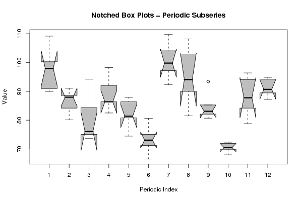
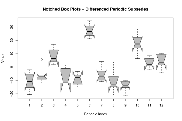
109,20 88,60 94,30 98,30 86,40 80,60 104,10 108,20 93,40 71,90 94,10 94,90 96,40 91,10 84,40 86,40 88,00 75,10 109,70 103,00 82,10 68,00 96,40 94,30 90,00 88,00 76,10 82,50 81,40 66,50 97,20 94,10 80,70 70,50 87,80 89,50 99,60 84,20 75,10 92,00 80,80 73,10 99,80 90,00 83,10 72,40 78,80 87,30 91,00 80,10 73,60 86,40 74,50 71,20 92,40 81,50 85,30 69,90 84,20 90,70 100,30 | |||||||||||||||||||||||||||||||
Tables (Output of Computation) | |||||||||||||||||||||||||||||||
| |||||||||||||||||||||||||||||||
Figures (Output of Computation) | |||||||||||||||||||||||||||||||
Input Parameters & R Code | |||||||||||||||||||||||||||||||
| Parameters (Session): | |||||||||||||||||||||||||||||||
| par1 = 12 ; | |||||||||||||||||||||||||||||||
| Parameters (R input): | |||||||||||||||||||||||||||||||
| par1 = 12 ; | |||||||||||||||||||||||||||||||
| R code (references can be found in the software module): | |||||||||||||||||||||||||||||||
par1 <- as.numeric(par1) | |||||||||||||||||||||||||||||||