Free Statistics
of Irreproducible Research!
Description of Statistical Computation | |||||||||||||||||||||
|---|---|---|---|---|---|---|---|---|---|---|---|---|---|---|---|---|---|---|---|---|---|
| Author's title | |||||||||||||||||||||
| Author | *The author of this computation has been verified* | ||||||||||||||||||||
| R Software Module | rwasp_meanplot.wasp | ||||||||||||||||||||
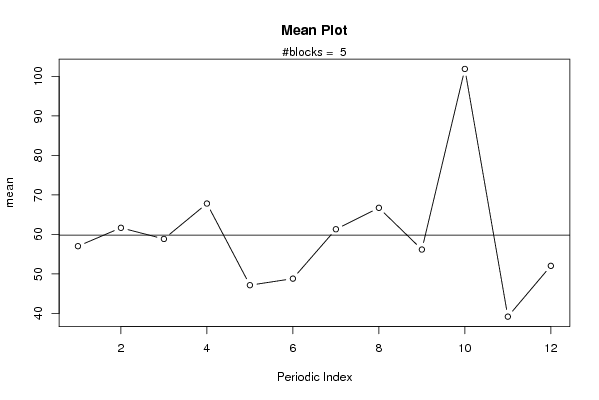
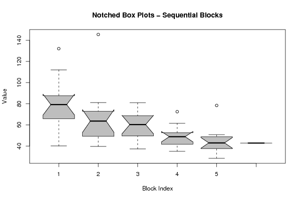
| Title produced by software | Mean Plot | ||||||||||||||||||||
| Date of computation | Mon, 03 Nov 2008 14:55:54 -0700 | ||||||||||||||||||||
| Cite this page as follows | Statistical Computations at FreeStatistics.org, Office for Research Development and Education, URL https://freestatistics.org/blog/index.php?v=date/2008/Nov/03/t1225749390jgcdpmemrmto16q.htm/, Retrieved Wed, 20 May 2026 17:40:20 +0000 | ||||||||||||||||||||
| Statistical Computations at FreeStatistics.org, Office for Research Development and Education, URL https://freestatistics.org/blog/index.php?pk=21339, Retrieved Wed, 20 May 2026 17:40:20 +0000 | |||||||||||||||||||||
| QR Codes: | |||||||||||||||||||||
|
| |||||||||||||||||||||
| Original text written by user: | |||||||||||||||||||||
| IsPrivate? | No (this computation is public) | ||||||||||||||||||||
| User-defined keywords | |||||||||||||||||||||
| Estimated Impact | 357 | ||||||||||||||||||||
Tree of Dependent Computations | |||||||||||||||||||||
| Family? (F = Feedback message, R = changed R code, M = changed R Module, P = changed Parameters, D = changed Data) | |||||||||||||||||||||
| F [Mean Plot] [workshop 3] [2007-10-26 12:14:28] [e9ffc5de6f8a7be62f22b142b5b6b1a8] F D [Mean Plot] [WS3 Q5] [2008-11-01 18:55:07] [74be16979710d4c4e7c6647856088456] F [Mean Plot] [T5] [2008-11-03 21:55:54] [e11d930c9e2984715c66c796cf63ef19] [Current] | |||||||||||||||||||||
| Feedback Forum | |||||||||||||||||||||
Post a new message | |||||||||||||||||||||
Dataset | |||||||||||||||||||||
| Dataseries X: | |||||||||||||||||||||
72,50 59,40 85,70 88,20 62,80 87,00 79,20 112,00 79,20 132,10 40,10 69,00 59,40 73,80 57,40 81,10 46,60 41,40 71,20 67,90 72,00 145,50 39,70 51,90 73,70 70,90 60,80 61,00 54,50 39,10 66,60 58,50 59,80 80,90 37,30 44,60 48,70 54,00 49,50 61,60 35,00 35,70 51,30 49,00 41,50 72,50 42,10 44,10 45,10 50,30 40,90 47,20 36,90 40,90 38,30 46,30 28,40 78,40 36,80 50,70 42,80 | |||||||||||||||||||||
Tables (Output of Computation) | |||||||||||||||||||||
| |||||||||||||||||||||
Figures (Output of Computation) | |||||||||||||||||||||
Input Parameters & R Code | |||||||||||||||||||||
| Parameters (Session): | |||||||||||||||||||||
| par1 = 12 ; | |||||||||||||||||||||
| Parameters (R input): | |||||||||||||||||||||
| par1 = 12 ; par2 = ; par3 = ; par4 = ; par5 = ; par6 = ; par7 = ; par8 = ; par9 = ; par10 = ; par11 = ; par12 = ; par13 = ; par14 = ; par15 = ; par16 = ; par17 = ; par18 = ; par19 = ; par20 = ; | |||||||||||||||||||||
| R code (references can be found in the software module): | |||||||||||||||||||||
par1 <- as.numeric(par1) | |||||||||||||||||||||