Free Statistics
of Irreproducible Research!
Description of Statistical Computation | |||||||||||||||||||||||||||||||||||||||||||||||||||||||||||||||||||||||||||||||||||||||||||||||||||||
|---|---|---|---|---|---|---|---|---|---|---|---|---|---|---|---|---|---|---|---|---|---|---|---|---|---|---|---|---|---|---|---|---|---|---|---|---|---|---|---|---|---|---|---|---|---|---|---|---|---|---|---|---|---|---|---|---|---|---|---|---|---|---|---|---|---|---|---|---|---|---|---|---|---|---|---|---|---|---|---|---|---|---|---|---|---|---|---|---|---|---|---|---|---|---|---|---|---|---|---|---|---|
| Author's title | |||||||||||||||||||||||||||||||||||||||||||||||||||||||||||||||||||||||||||||||||||||||||||||||||||||
| Author | *The author of this computation has been verified* | ||||||||||||||||||||||||||||||||||||||||||||||||||||||||||||||||||||||||||||||||||||||||||||||||||||
| R Software Module | rwasp_notchedbox1.wasp | ||||||||||||||||||||||||||||||||||||||||||||||||||||||||||||||||||||||||||||||||||||||||||||||||||||
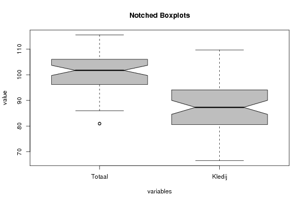
| Title produced by software | Notched Boxplots | ||||||||||||||||||||||||||||||||||||||||||||||||||||||||||||||||||||||||||||||||||||||||||||||||||||
| Date of computation | Mon, 03 Nov 2008 02:57:32 -0700 | ||||||||||||||||||||||||||||||||||||||||||||||||||||||||||||||||||||||||||||||||||||||||||||||||||||
| Cite this page as follows | Statistical Computations at FreeStatistics.org, Office for Research Development and Education, URL https://freestatistics.org/blog/index.php?v=date/2008/Nov/03/t1225706312frwqf5gkh5h41rr.htm/, Retrieved Sat, 23 May 2026 05:36:44 +0000 | ||||||||||||||||||||||||||||||||||||||||||||||||||||||||||||||||||||||||||||||||||||||||||||||||||||
| Statistical Computations at FreeStatistics.org, Office for Research Development and Education, URL https://freestatistics.org/blog/index.php?pk=20781, Retrieved Sat, 23 May 2026 05:36:44 +0000 | |||||||||||||||||||||||||||||||||||||||||||||||||||||||||||||||||||||||||||||||||||||||||||||||||||||
| QR Codes: | |||||||||||||||||||||||||||||||||||||||||||||||||||||||||||||||||||||||||||||||||||||||||||||||||||||
|
| |||||||||||||||||||||||||||||||||||||||||||||||||||||||||||||||||||||||||||||||||||||||||||||||||||||
| Original text written by user: | |||||||||||||||||||||||||||||||||||||||||||||||||||||||||||||||||||||||||||||||||||||||||||||||||||||
| IsPrivate? | No (this computation is public) | ||||||||||||||||||||||||||||||||||||||||||||||||||||||||||||||||||||||||||||||||||||||||||||||||||||
| User-defined keywords | |||||||||||||||||||||||||||||||||||||||||||||||||||||||||||||||||||||||||||||||||||||||||||||||||||||
| Estimated Impact | 584 | ||||||||||||||||||||||||||||||||||||||||||||||||||||||||||||||||||||||||||||||||||||||||||||||||||||
Tree of Dependent Computations | |||||||||||||||||||||||||||||||||||||||||||||||||||||||||||||||||||||||||||||||||||||||||||||||||||||
| Family? (F = Feedback message, R = changed R code, M = changed R Module, P = changed Parameters, D = changed Data) | |||||||||||||||||||||||||||||||||||||||||||||||||||||||||||||||||||||||||||||||||||||||||||||||||||||
| F [Notched Boxplots] [workshop 3] [2007-10-26 13:31:48] [e9ffc5de6f8a7be62f22b142b5b6b1a8] F D [Notched Boxplots] [Q1 - Notched Boxplot] [2008-11-03 09:57:32] [f1a30f1149cef3ef3ef69d586c6c3c1c] [Current] - D [Notched Boxplots] [Task 2 - Notched ...] [2008-11-03 10:42:59] [a7f04e0e73ce3683561193958d653479] F D [Notched Boxplots] [Task 2 - Notched ...] [2008-11-03 10:48:16] [a7f04e0e73ce3683561193958d653479] F RMPD [Kendall tau Correlation Matrix] [EDA Part 2 - Q1 ] [2008-11-03 19:39:18] [a7f04e0e73ce3683561193958d653479] F RMPD [Star Plot] [EDA Part 2 - Q2] [2008-11-03 19:59:24] [a7f04e0e73ce3683561193958d653479] F D [Notched Boxplots] [EDA Part 2 - Q3] [2008-11-03 20:15:28] [a7f04e0e73ce3683561193958d653479] - R [Notched Boxplots] [Task 3 - Reducing...] [2008-11-03 20:15:16] [a7f04e0e73ce3683561193958d653479] F D [Notched Boxplots] [Task 3 - Reducing...] [2008-11-03 20:22:30] [1d988b04e8982749ec309eda662241b4] F D [Notched Boxplots] [Notched Boxplots ...] [2008-11-03 23:11:44] [fce9014b1ad8484790f3b34d6ba09f7b] - [Notched Boxplots] [] [2008-11-10 11:10:34] [888addc516c3b812dd7be4bd54caa358] - RMPD [Testing Variance - p-value (probability)] [Various types of ...] [2008-11-11 12:12:50] [a7f04e0e73ce3683561193958d653479] - P [Testing Variance - p-value (probability)] [Various types of ...] [2008-11-11 19:15:52] [a7f04e0e73ce3683561193958d653479] F RMPD [Bivariate Kernel Density Estimation] [Various EDA topic...] [2008-11-11 13:04:27] [a7f04e0e73ce3683561193958d653479] F D [Bivariate Kernel Density Estimation] [Various EDA topic...] [2008-11-11 13:51:35] [a7f04e0e73ce3683561193958d653479] F RMPD [Hierarchical Clustering] [Various EDA topic...] [2008-11-11 14:17:41] [a7f04e0e73ce3683561193958d653479] F RMPD [Bivariate Kernel Density Estimation] [Various EDA topic...] [2008-11-11 13:11:59] [a7f04e0e73ce3683561193958d653479] - D [Notched Boxplots] [Notched boxplots:...] [2008-12-08 19:48:56] [a7f04e0e73ce3683561193958d653479] - D [Notched Boxplots] [Notched Boxplots:...] [2008-12-08 19:57:25] [a7f04e0e73ce3683561193958d653479] - D [Notched Boxplots] [Notched Boxplots:...] [2008-12-08 20:08:07] [a7f04e0e73ce3683561193958d653479] - RMPD [Bivariate Kernel Density Estimation] [Bivariate Kernel ...] [2008-12-08 20:23:10] [a7f04e0e73ce3683561193958d653479] - D [Bivariate Kernel Density Estimation] [Bivariate Kernel ...] [2008-12-08 20:26:55] [a7f04e0e73ce3683561193958d653479] - D [Bivariate Kernel Density Estimation] [Bivariate Kernel ...] [2008-12-08 20:30:45] [a7f04e0e73ce3683561193958d653479] - PD [Bivariate Kernel Density Estimation] [Bivariate Kernel ...] [2008-12-08 21:50:20] [a7f04e0e73ce3683561193958d653479] - RMPD [Trivariate Scatterplots] [Trivariate Scatte...] [2008-12-08 20:42:07] [a7f04e0e73ce3683561193958d653479] - PD [Trivariate Scatterplots] [Trivariate Scatte...] [2008-12-08 20:47:38] [a7f04e0e73ce3683561193958d653479] - RMPD [Box-Cox Linearity Plot] [Bow-Cox Linearity...] [2008-12-08 20:57:51] [a7f04e0e73ce3683561193958d653479] - D [Box-Cox Linearity Plot] [Box-Cox Linearity...] [2008-12-08 21:02:17] [a7f04e0e73ce3683561193958d653479] - D [Box-Cox Linearity Plot] [Box-Cox Linearity...] [2008-12-16 20:21:18] [a7f04e0e73ce3683561193958d653479] - D [Notched Boxplots] [Notched boxplots:...] [2008-12-16 19:16:07] [a7f04e0e73ce3683561193958d653479] | |||||||||||||||||||||||||||||||||||||||||||||||||||||||||||||||||||||||||||||||||||||||||||||||||||||
| Feedback Forum | |||||||||||||||||||||||||||||||||||||||||||||||||||||||||||||||||||||||||||||||||||||||||||||||||||||
Post a new message | |||||||||||||||||||||||||||||||||||||||||||||||||||||||||||||||||||||||||||||||||||||||||||||||||||||
Dataset | |||||||||||||||||||||||||||||||||||||||||||||||||||||||||||||||||||||||||||||||||||||||||||||||||||||
| Dataseries X: | |||||||||||||||||||||||||||||||||||||||||||||||||||||||||||||||||||||||||||||||||||||||||||||||||||||
110.40 109.20 96.40 88.60 101.90 94.30 106.20 98.30 81.00 86.40 94.70 80.60 101.00 104.10 109.40 108.20 102.30 93.40 90.70 71.90 96.20 94.10 96.10 94.90 106.00 96.40 103.10 91.10 102.00 84.40 104.70 86.40 86.00 88.00 92.10 75.10 106.90 109.70 112.60 103.00 101.70 82.10 92.00 68.00 97.40 96.40 97.00 94.30 105.40 90.00 102.70 88.00 98.10 76.10 104.50 82.50 87.40 81.40 89.90 66.50 109.80 97.20 111.70 94.10 98.60 80.70 96.90 70.50 95.10 87.80 97.00 89.50 112.70 99.60 102.90 84.20 97.40 75.10 111.40 92.00 87.40 80.80 96.80 73.10 114.10 99.80 110.30 90.00 103.90 83.10 101.60 72.40 94.60 78.80 95.90 87.30 104.70 91.00 102.80 80.10 98.10 73.60 113.90 86.40 80.90 74.50 95.70 71.20 113.20 92.40 105.90 81.50 108.80 85.30 102.30 69.90 99.00 84.20 100.70 90.70 115.50 100.30 | |||||||||||||||||||||||||||||||||||||||||||||||||||||||||||||||||||||||||||||||||||||||||||||||||||||
Tables (Output of Computation) | |||||||||||||||||||||||||||||||||||||||||||||||||||||||||||||||||||||||||||||||||||||||||||||||||||||
| |||||||||||||||||||||||||||||||||||||||||||||||||||||||||||||||||||||||||||||||||||||||||||||||||||||
Figures (Output of Computation) | |||||||||||||||||||||||||||||||||||||||||||||||||||||||||||||||||||||||||||||||||||||||||||||||||||||
Input Parameters & R Code | |||||||||||||||||||||||||||||||||||||||||||||||||||||||||||||||||||||||||||||||||||||||||||||||||||||
| Parameters (Session): | |||||||||||||||||||||||||||||||||||||||||||||||||||||||||||||||||||||||||||||||||||||||||||||||||||||
| par1 = grey ; | |||||||||||||||||||||||||||||||||||||||||||||||||||||||||||||||||||||||||||||||||||||||||||||||||||||
| Parameters (R input): | |||||||||||||||||||||||||||||||||||||||||||||||||||||||||||||||||||||||||||||||||||||||||||||||||||||
| par1 = grey ; | |||||||||||||||||||||||||||||||||||||||||||||||||||||||||||||||||||||||||||||||||||||||||||||||||||||
| R code (references can be found in the software module): | |||||||||||||||||||||||||||||||||||||||||||||||||||||||||||||||||||||||||||||||||||||||||||||||||||||
z <- as.data.frame(t(y)) | |||||||||||||||||||||||||||||||||||||||||||||||||||||||||||||||||||||||||||||||||||||||||||||||||||||