Repository of Reproducible Computations

Free Statistics

of Irreproducible Research!

Author's title

Author

*Unverified author*

R Software Module

rwasp_autocorrelation.wasp

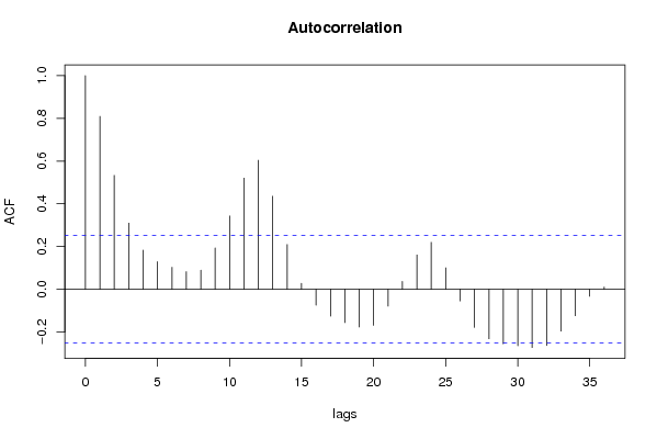
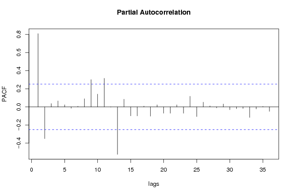
Title produced by software

(Partial) Autocorrelation Function

Date of computation

Wed, 24 Dec 2008 05:57:31 -0700

Cite this page as follows

Statistical Computations at FreeStatistics.org, Office for Research Development and Education, URL https://freestatistics.org/blog/index.php?v=date/2008/Dec/24/t1230123489x14t0qdg5vdfz54.htm/, Retrieved Fri, 24 May 2024 18:11:41 +0000

Statistical Computations at FreeStatistics.org, Office for Research Development and Education, URL https://freestatistics.org/blog/index.php?pk=36539, Retrieved Fri, 24 May 2024 18:11:41 +0000

QR Codes:

Paste this QR Code to cite your computation.

Original text written by user:

IsPrivate?

No (this computation is public)

User-defined keywords

Estimated Impact

230

Family? (F = Feedback message, R = changed R code, M = changed R Module, P = changed Parameters, D = changed Data)

-     [Univariate Data Series] [data set] [2008-12-01 19:54:57] [b98453cac15ba1066b407e146608df68]
F RMP   [Standard Deviation-Mean Plot] [q1] [2008-12-08 12:37:39] [3ffd109c9e040b1ae7e5dbe576d4698c]
F    D    [Standard Deviation-Mean Plot] [SMP] [2008-12-08 12:41:29] [3ffd109c9e040b1ae7e5dbe576d4698c]
- RM        [Variance Reduction Matrix] [VRM] [2008-12-08 13:10:17] [3ffd109c9e040b1ae7e5dbe576d4698c]
- RM          [(Partial) Autocorrelation Function] [ACF] [2008-12-08 13:14:12] [3ffd109c9e040b1ae7e5dbe576d4698c]
F               [(Partial) Autocorrelation Function] [ACF] [2008-12-08 13:16:18] [3ffd109c9e040b1ae7e5dbe576d4698c]
- R P             [(Partial) Autocorrelation Function] [ACF] [2008-12-18 16:25:12] [3ffd109c9e040b1ae7e5dbe576d4698c]
-   P                 [(Partial) Autocorrelation Function] [ACF] [2008-12-24 12:57:31] [c00776cbed2786c9c4960950021bd861] [Current]

Feedback Forum

Post a new message

Dataseries X:

Download CSV

Histogram

Boxplots

Summary of computational transaction
Raw Input	view raw input (R code)
Raw Output	view raw output of R engine
Computing time	1 seconds
R Server	'George Udny Yule' @ 72.249.76.132

\begin{tabular}{lllllllll}
\hline
Summary of computational transaction \tabularnewline
Raw Input & view raw input (R code)  \tabularnewline
Raw Output & view raw output of R engine  \tabularnewline
Computing time & 1 seconds \tabularnewline
R Server & 'George Udny Yule' @ 72.249.76.132 \tabularnewline
\hline
\end{tabular}
%Source: https://freestatistics.org/blog/index.php?pk=36539&T=0

[TABLE]
[ROW][C]Summary of computational transaction[/C][/ROW]
[ROW][C]Raw Input[/C][C]view raw input (R code) [/C][/ROW]
[ROW][C]Raw Output[/C][C]view raw output of R engine [/C][/ROW]
[ROW][C]Computing time[/C][C]1 seconds[/C][/ROW]
[ROW][C]R Server[/C][C]'George Udny Yule' @ 72.249.76.132[/C][/ROW]
[/TABLE]
Source: https://freestatistics.org/blog/index.php?pk=36539&T=0

Globally Unique Identifier (entire table): ba.freestatistics.org/blog/index.php?pk=36539&T=0

As an alternative you can also use a QR Code:

The GUIDs for individual cells are displayed in the table below:

Summary of computational transaction
Raw Input	view raw input (R code)
Raw Output	view raw output of R engine
Computing time	1 seconds
R Server	'George Udny Yule' @ 72.249.76.132

Autocorrelation Function
Time lag k	ACF(k)	T-STAT	P-value
1	0.809251	6.3205	0
2	0.533477	4.1666	5e-05
3	0.309871	2.4202	0.009253
4	0.183137	1.4303	0.07886
5	0.129405	1.0107	0.158079
6	0.102599	0.8013	0.213028
7	0.082375	0.6434	0.261198
8	0.089375	0.698	0.243902
9	0.193641	1.5124	0.0678
10	0.343131	2.6799	0.004727
11	0.520575	4.0658	7e-05
12	0.603667	4.7148	7e-06
13	0.435778	3.4035	0.00059
14	0.209656	1.6375	0.053341
15	0.027427	0.2142	0.415548
16	-0.074432	-0.5813	0.281579
17	-0.125685	-0.9816	0.165079
18	-0.155777	-1.2167	0.114211
19	-0.176501	-1.3785	0.08654
20	-0.168619	-1.317	0.096389
21	-0.078756	-0.6151	0.270386
22	0.036598	0.2858	0.387985
23	0.160877	1.2565	0.106865
24	0.219544	1.7147	0.045739
25	0.100052	0.7814	0.218786
26	-0.05472	-0.4274	0.335304
27	-0.178398	-1.3933	0.084288
28	-0.231905	-1.8112	0.037515
29	-0.255854	-1.9983	0.025074
30	-0.26482	-2.0683	0.021429
31	-0.272707	-2.1299	0.018611
32	-0.263338	-2.0567	0.021998
33	-0.196039	-1.5311	0.065456
34	-0.124055	-0.9689	0.16821
35	-0.032923	-0.2571	0.39897
36	0.010205	0.0797	0.468368

\begin{tabular}{lllllllll}
\hline
Autocorrelation Function \tabularnewline
Time lag k & ACF(k) & T-STAT & P-value \tabularnewline
1 & 0.809251 & 6.3205 & 0 \tabularnewline
2 & 0.533477 & 4.1666 & 5e-05 \tabularnewline
3 & 0.309871 & 2.4202 & 0.009253 \tabularnewline
4 & 0.183137 & 1.4303 & 0.07886 \tabularnewline
5 & 0.129405 & 1.0107 & 0.158079 \tabularnewline
6 & 0.102599 & 0.8013 & 0.213028 \tabularnewline
7 & 0.082375 & 0.6434 & 0.261198 \tabularnewline
8 & 0.089375 & 0.698 & 0.243902 \tabularnewline
9 & 0.193641 & 1.5124 & 0.0678 \tabularnewline
10 & 0.343131 & 2.6799 & 0.004727 \tabularnewline
11 & 0.520575 & 4.0658 & 7e-05 \tabularnewline
12 & 0.603667 & 4.7148 & 7e-06 \tabularnewline
13 & 0.435778 & 3.4035 & 0.00059 \tabularnewline
14 & 0.209656 & 1.6375 & 0.053341 \tabularnewline
15 & 0.027427 & 0.2142 & 0.415548 \tabularnewline
16 & -0.074432 & -0.5813 & 0.281579 \tabularnewline
17 & -0.125685 & -0.9816 & 0.165079 \tabularnewline
18 & -0.155777 & -1.2167 & 0.114211 \tabularnewline
19 & -0.176501 & -1.3785 & 0.08654 \tabularnewline
20 & -0.168619 & -1.317 & 0.096389 \tabularnewline
21 & -0.078756 & -0.6151 & 0.270386 \tabularnewline
22 & 0.036598 & 0.2858 & 0.387985 \tabularnewline
23 & 0.160877 & 1.2565 & 0.106865 \tabularnewline
24 & 0.219544 & 1.7147 & 0.045739 \tabularnewline
25 & 0.100052 & 0.7814 & 0.218786 \tabularnewline
26 & -0.05472 & -0.4274 & 0.335304 \tabularnewline
27 & -0.178398 & -1.3933 & 0.084288 \tabularnewline
28 & -0.231905 & -1.8112 & 0.037515 \tabularnewline
29 & -0.255854 & -1.9983 & 0.025074 \tabularnewline
30 & -0.26482 & -2.0683 & 0.021429 \tabularnewline
31 & -0.272707 & -2.1299 & 0.018611 \tabularnewline
32 & -0.263338 & -2.0567 & 0.021998 \tabularnewline
33 & -0.196039 & -1.5311 & 0.065456 \tabularnewline
34 & -0.124055 & -0.9689 & 0.16821 \tabularnewline
35 & -0.032923 & -0.2571 & 0.39897 \tabularnewline
36 & 0.010205 & 0.0797 & 0.468368 \tabularnewline
\hline
\end{tabular}
%Source: https://freestatistics.org/blog/index.php?pk=36539&T=1

[TABLE]
[ROW][C]Autocorrelation Function[/C][/ROW]
[ROW][C]Time lag k[/C][C]ACF(k)[/C][C]T-STAT[/C][C]P-value[/C][/ROW]
[ROW][C]1[/C][C]0.809251[/C][C]6.3205[/C][C]0[/C][/ROW]
[ROW][C]2[/C][C]0.533477[/C][C]4.1666[/C][C]5e-05[/C][/ROW]
[ROW][C]3[/C][C]0.309871[/C][C]2.4202[/C][C]0.009253[/C][/ROW]
[ROW][C]4[/C][C]0.183137[/C][C]1.4303[/C][C]0.07886[/C][/ROW]
[ROW][C]5[/C][C]0.129405[/C][C]1.0107[/C][C]0.158079[/C][/ROW]
[ROW][C]6[/C][C]0.102599[/C][C]0.8013[/C][C]0.213028[/C][/ROW]
[ROW][C]7[/C][C]0.082375[/C][C]0.6434[/C][C]0.261198[/C][/ROW]
[ROW][C]8[/C][C]0.089375[/C][C]0.698[/C][C]0.243902[/C][/ROW]
[ROW][C]9[/C][C]0.193641[/C][C]1.5124[/C][C]0.0678[/C][/ROW]
[ROW][C]10[/C][C]0.343131[/C][C]2.6799[/C][C]0.004727[/C][/ROW]
[ROW][C]11[/C][C]0.520575[/C][C]4.0658[/C][C]7e-05[/C][/ROW]
[ROW][C]12[/C][C]0.603667[/C][C]4.7148[/C][C]7e-06[/C][/ROW]
[ROW][C]13[/C][C]0.435778[/C][C]3.4035[/C][C]0.00059[/C][/ROW]
[ROW][C]14[/C][C]0.209656[/C][C]1.6375[/C][C]0.053341[/C][/ROW]
[ROW][C]15[/C][C]0.027427[/C][C]0.2142[/C][C]0.415548[/C][/ROW]
[ROW][C]16[/C][C]-0.074432[/C][C]-0.5813[/C][C]0.281579[/C][/ROW]
[ROW][C]17[/C][C]-0.125685[/C][C]-0.9816[/C][C]0.165079[/C][/ROW]
[ROW][C]18[/C][C]-0.155777[/C][C]-1.2167[/C][C]0.114211[/C][/ROW]
[ROW][C]19[/C][C]-0.176501[/C][C]-1.3785[/C][C]0.08654[/C][/ROW]
[ROW][C]20[/C][C]-0.168619[/C][C]-1.317[/C][C]0.096389[/C][/ROW]
[ROW][C]21[/C][C]-0.078756[/C][C]-0.6151[/C][C]0.270386[/C][/ROW]
[ROW][C]22[/C][C]0.036598[/C][C]0.2858[/C][C]0.387985[/C][/ROW]
[ROW][C]23[/C][C]0.160877[/C][C]1.2565[/C][C]0.106865[/C][/ROW]
[ROW][C]24[/C][C]0.219544[/C][C]1.7147[/C][C]0.045739[/C][/ROW]
[ROW][C]25[/C][C]0.100052[/C][C]0.7814[/C][C]0.218786[/C][/ROW]
[ROW][C]26[/C][C]-0.05472[/C][C]-0.4274[/C][C]0.335304[/C][/ROW]
[ROW][C]27[/C][C]-0.178398[/C][C]-1.3933[/C][C]0.084288[/C][/ROW]
[ROW][C]28[/C][C]-0.231905[/C][C]-1.8112[/C][C]0.037515[/C][/ROW]
[ROW][C]29[/C][C]-0.255854[/C][C]-1.9983[/C][C]0.025074[/C][/ROW]
[ROW][C]30[/C][C]-0.26482[/C][C]-2.0683[/C][C]0.021429[/C][/ROW]
[ROW][C]31[/C][C]-0.272707[/C][C]-2.1299[/C][C]0.018611[/C][/ROW]
[ROW][C]32[/C][C]-0.263338[/C][C]-2.0567[/C][C]0.021998[/C][/ROW]
[ROW][C]33[/C][C]-0.196039[/C][C]-1.5311[/C][C]0.065456[/C][/ROW]
[ROW][C]34[/C][C]-0.124055[/C][C]-0.9689[/C][C]0.16821[/C][/ROW]
[ROW][C]35[/C][C]-0.032923[/C][C]-0.2571[/C][C]0.39897[/C][/ROW]
[ROW][C]36[/C][C]0.010205[/C][C]0.0797[/C][C]0.468368[/C][/ROW]
[/TABLE]
Source: https://freestatistics.org/blog/index.php?pk=36539&T=1

Globally Unique Identifier (entire table): ba.freestatistics.org/blog/index.php?pk=36539&T=1

As an alternative you can also use a QR Code:

The GUIDs for individual cells are displayed in the table below:

Autocorrelation Function
Time lag k	ACF(k)	T-STAT	P-value
1	0.809251	6.3205	0
2	0.533477	4.1666	5e-05
3	0.309871	2.4202	0.009253
4	0.183137	1.4303	0.07886
5	0.129405	1.0107	0.158079
6	0.102599	0.8013	0.213028
7	0.082375	0.6434	0.261198
8	0.089375	0.698	0.243902
9	0.193641	1.5124	0.0678
10	0.343131	2.6799	0.004727
11	0.520575	4.0658	7e-05
12	0.603667	4.7148	7e-06
13	0.435778	3.4035	0.00059
14	0.209656	1.6375	0.053341
15	0.027427	0.2142	0.415548
16	-0.074432	-0.5813	0.281579
17	-0.125685	-0.9816	0.165079
18	-0.155777	-1.2167	0.114211
19	-0.176501	-1.3785	0.08654
20	-0.168619	-1.317	0.096389
21	-0.078756	-0.6151	0.270386
22	0.036598	0.2858	0.387985
23	0.160877	1.2565	0.106865
24	0.219544	1.7147	0.045739
25	0.100052	0.7814	0.218786
26	-0.05472	-0.4274	0.335304
27	-0.178398	-1.3933	0.084288
28	-0.231905	-1.8112	0.037515
29	-0.255854	-1.9983	0.025074
30	-0.26482	-2.0683	0.021429
31	-0.272707	-2.1299	0.018611
32	-0.263338	-2.0567	0.021998
33	-0.196039	-1.5311	0.065456
34	-0.124055	-0.9689	0.16821
35	-0.032923	-0.2571	0.39897
36	0.010205	0.0797	0.468368

Partial Autocorrelation Function
Time lag k	PACF(k)	T-STAT	P-value
1	0.809251	6.3205	0
2	-0.351802	-2.7477	0.003941
3	0.036281	0.2834	0.388929
4	0.065199	0.5092	0.306217
5	0.023071	0.1802	0.428802
6	-0.015319	-0.1196	0.45258
7	0.006532	0.051	0.479739
8	0.089447	0.6986	0.243728
9	0.300694	2.3485	0.011053
10	0.14091	1.1005	0.137711
11	0.315416	2.4635	0.008298
12	-0.003528	-0.0276	0.489054
13	-0.52514	-4.1015	6.2e-05
14	0.084565	0.6605	0.255717
15	-0.099732	-0.7789	0.219516
16	-0.100706	-0.7865	0.217299
17	0.008247	0.0644	0.474427
18	-0.10309	-0.8052	0.211927
19	0.02208	0.1725	0.431826
20	-0.070018	-0.5469	0.293235
21	-0.07108	-0.5552	0.290411
22	0.022292	0.1741	0.431179
23	-0.070982	-0.5544	0.29067
24	0.116768	0.912	0.182684
25	-0.107724	-0.8414	0.201718
26	0.051761	0.4043	0.343717
27	0.010509	0.0821	0.467427
28	-0.011316	-0.0884	0.464933
29	0.0319	0.2491	0.402043
30	-0.031533	-0.2463	0.403146
31	-0.020622	-0.1611	0.436287
32	-0.018484	-0.1444	0.442844
33	-0.117348	-0.9165	0.181503
34	-0.023533	-0.1838	0.42739
35	0.004817	0.0376	0.485055
36	-0.049656	-0.3878	0.349748

\begin{tabular}{lllllllll}
\hline
Partial Autocorrelation Function \tabularnewline
Time lag k & PACF(k) & T-STAT & P-value \tabularnewline
1 & 0.809251 & 6.3205 & 0 \tabularnewline
2 & -0.351802 & -2.7477 & 0.003941 \tabularnewline
3 & 0.036281 & 0.2834 & 0.388929 \tabularnewline
4 & 0.065199 & 0.5092 & 0.306217 \tabularnewline
5 & 0.023071 & 0.1802 & 0.428802 \tabularnewline
6 & -0.015319 & -0.1196 & 0.45258 \tabularnewline
7 & 0.006532 & 0.051 & 0.479739 \tabularnewline
8 & 0.089447 & 0.6986 & 0.243728 \tabularnewline
9 & 0.300694 & 2.3485 & 0.011053 \tabularnewline
10 & 0.14091 & 1.1005 & 0.137711 \tabularnewline
11 & 0.315416 & 2.4635 & 0.008298 \tabularnewline
12 & -0.003528 & -0.0276 & 0.489054 \tabularnewline
13 & -0.52514 & -4.1015 & 6.2e-05 \tabularnewline
14 & 0.084565 & 0.6605 & 0.255717 \tabularnewline
15 & -0.099732 & -0.7789 & 0.219516 \tabularnewline
16 & -0.100706 & -0.7865 & 0.217299 \tabularnewline
17 & 0.008247 & 0.0644 & 0.474427 \tabularnewline
18 & -0.10309 & -0.8052 & 0.211927 \tabularnewline
19 & 0.02208 & 0.1725 & 0.431826 \tabularnewline
20 & -0.070018 & -0.5469 & 0.293235 \tabularnewline
21 & -0.07108 & -0.5552 & 0.290411 \tabularnewline
22 & 0.022292 & 0.1741 & 0.431179 \tabularnewline
23 & -0.070982 & -0.5544 & 0.29067 \tabularnewline
24 & 0.116768 & 0.912 & 0.182684 \tabularnewline
25 & -0.107724 & -0.8414 & 0.201718 \tabularnewline
26 & 0.051761 & 0.4043 & 0.343717 \tabularnewline
27 & 0.010509 & 0.0821 & 0.467427 \tabularnewline
28 & -0.011316 & -0.0884 & 0.464933 \tabularnewline
29 & 0.0319 & 0.2491 & 0.402043 \tabularnewline
30 & -0.031533 & -0.2463 & 0.403146 \tabularnewline
31 & -0.020622 & -0.1611 & 0.436287 \tabularnewline
32 & -0.018484 & -0.1444 & 0.442844 \tabularnewline
33 & -0.117348 & -0.9165 & 0.181503 \tabularnewline
34 & -0.023533 & -0.1838 & 0.42739 \tabularnewline
35 & 0.004817 & 0.0376 & 0.485055 \tabularnewline
36 & -0.049656 & -0.3878 & 0.349748 \tabularnewline
\hline
\end{tabular}
%Source: https://freestatistics.org/blog/index.php?pk=36539&T=2

[TABLE]
[ROW][C]Partial Autocorrelation Function[/C][/ROW]
[ROW][C]Time lag k[/C][C]PACF(k)[/C][C]T-STAT[/C][C]P-value[/C][/ROW]
[ROW][C]1[/C][C]0.809251[/C][C]6.3205[/C][C]0[/C][/ROW]
[ROW][C]2[/C][C]-0.351802[/C][C]-2.7477[/C][C]0.003941[/C][/ROW]
[ROW][C]3[/C][C]0.036281[/C][C]0.2834[/C][C]0.388929[/C][/ROW]
[ROW][C]4[/C][C]0.065199[/C][C]0.5092[/C][C]0.306217[/C][/ROW]
[ROW][C]5[/C][C]0.023071[/C][C]0.1802[/C][C]0.428802[/C][/ROW]
[ROW][C]6[/C][C]-0.015319[/C][C]-0.1196[/C][C]0.45258[/C][/ROW]
[ROW][C]7[/C][C]0.006532[/C][C]0.051[/C][C]0.479739[/C][/ROW]
[ROW][C]8[/C][C]0.089447[/C][C]0.6986[/C][C]0.243728[/C][/ROW]
[ROW][C]9[/C][C]0.300694[/C][C]2.3485[/C][C]0.011053[/C][/ROW]
[ROW][C]10[/C][C]0.14091[/C][C]1.1005[/C][C]0.137711[/C][/ROW]
[ROW][C]11[/C][C]0.315416[/C][C]2.4635[/C][C]0.008298[/C][/ROW]
[ROW][C]12[/C][C]-0.003528[/C][C]-0.0276[/C][C]0.489054[/C][/ROW]
[ROW][C]13[/C][C]-0.52514[/C][C]-4.1015[/C][C]6.2e-05[/C][/ROW]
[ROW][C]14[/C][C]0.084565[/C][C]0.6605[/C][C]0.255717[/C][/ROW]
[ROW][C]15[/C][C]-0.099732[/C][C]-0.7789[/C][C]0.219516[/C][/ROW]
[ROW][C]16[/C][C]-0.100706[/C][C]-0.7865[/C][C]0.217299[/C][/ROW]
[ROW][C]17[/C][C]0.008247[/C][C]0.0644[/C][C]0.474427[/C][/ROW]
[ROW][C]18[/C][C]-0.10309[/C][C]-0.8052[/C][C]0.211927[/C][/ROW]
[ROW][C]19[/C][C]0.02208[/C][C]0.1725[/C][C]0.431826[/C][/ROW]
[ROW][C]20[/C][C]-0.070018[/C][C]-0.5469[/C][C]0.293235[/C][/ROW]
[ROW][C]21[/C][C]-0.07108[/C][C]-0.5552[/C][C]0.290411[/C][/ROW]
[ROW][C]22[/C][C]0.022292[/C][C]0.1741[/C][C]0.431179[/C][/ROW]
[ROW][C]23[/C][C]-0.070982[/C][C]-0.5544[/C][C]0.29067[/C][/ROW]
[ROW][C]24[/C][C]0.116768[/C][C]0.912[/C][C]0.182684[/C][/ROW]
[ROW][C]25[/C][C]-0.107724[/C][C]-0.8414[/C][C]0.201718[/C][/ROW]
[ROW][C]26[/C][C]0.051761[/C][C]0.4043[/C][C]0.343717[/C][/ROW]
[ROW][C]27[/C][C]0.010509[/C][C]0.0821[/C][C]0.467427[/C][/ROW]
[ROW][C]28[/C][C]-0.011316[/C][C]-0.0884[/C][C]0.464933[/C][/ROW]
[ROW][C]29[/C][C]0.0319[/C][C]0.2491[/C][C]0.402043[/C][/ROW]
[ROW][C]30[/C][C]-0.031533[/C][C]-0.2463[/C][C]0.403146[/C][/ROW]
[ROW][C]31[/C][C]-0.020622[/C][C]-0.1611[/C][C]0.436287[/C][/ROW]
[ROW][C]32[/C][C]-0.018484[/C][C]-0.1444[/C][C]0.442844[/C][/ROW]
[ROW][C]33[/C][C]-0.117348[/C][C]-0.9165[/C][C]0.181503[/C][/ROW]
[ROW][C]34[/C][C]-0.023533[/C][C]-0.1838[/C][C]0.42739[/C][/ROW]
[ROW][C]35[/C][C]0.004817[/C][C]0.0376[/C][C]0.485055[/C][/ROW]
[ROW][C]36[/C][C]-0.049656[/C][C]-0.3878[/C][C]0.349748[/C][/ROW]
[/TABLE]
Source: https://freestatistics.org/blog/index.php?pk=36539&T=2

Globally Unique Identifier (entire table): ba.freestatistics.org/blog/index.php?pk=36539&T=2

As an alternative you can also use a QR Code:

The GUIDs for individual cells are displayed in the table below:

Partial Autocorrelation Function
Time lag k	PACF(k)	T-STAT	P-value
1	0.809251	6.3205	0
2	-0.351802	-2.7477	0.003941
3	0.036281	0.2834	0.388929
4	0.065199	0.5092	0.306217
5	0.023071	0.1802	0.428802
6	-0.015319	-0.1196	0.45258
7	0.006532	0.051	0.479739
8	0.089447	0.6986	0.243728
9	0.300694	2.3485	0.011053
10	0.14091	1.1005	0.137711
11	0.315416	2.4635	0.008298
12	-0.003528	-0.0276	0.489054
13	-0.52514	-4.1015	6.2e-05
14	0.084565	0.6605	0.255717
15	-0.099732	-0.7789	0.219516
16	-0.100706	-0.7865	0.217299
17	0.008247	0.0644	0.474427
18	-0.10309	-0.8052	0.211927
19	0.02208	0.1725	0.431826
20	-0.070018	-0.5469	0.293235
21	-0.07108	-0.5552	0.290411
22	0.022292	0.1741	0.431179
23	-0.070982	-0.5544	0.29067
24	0.116768	0.912	0.182684
25	-0.107724	-0.8414	0.201718
26	0.051761	0.4043	0.343717
27	0.010509	0.0821	0.467427
28	-0.011316	-0.0884	0.464933
29	0.0319	0.2491	0.402043
30	-0.031533	-0.2463	0.403146
31	-0.020622	-0.1611	0.436287
32	-0.018484	-0.1444	0.442844
33	-0.117348	-0.9165	0.181503
34	-0.023533	-0.1838	0.42739
35	0.004817	0.0376	0.485055
36	-0.049656	-0.3878	0.349748

Figure 1

PNG link

Postscript link

PDF link

Figure 2

PNG link

Postscript link

PDF link

Parameters (Session):

par1 = 36 ; par2 = 0.0 ; par3 = 0 ; par4 = 0 ; par5 = 12 ;

Parameters (R input):

par1 = 36 ; par2 = 0.0 ; par3 = 0 ; par4 = 0 ; par5 = 12 ;

R code (references can be found in the software module):

if (par1 == 'Default') {
par1 = 10*log10(length(x))
} else {
par1 <- as.numeric(par1)
}
par2 <- as.numeric(par2)
par3 <- as.numeric(par3)
par4 <- as.numeric(par4)
par5 <- as.numeric(par5)
if (par2 == 0) {
x <- log(x)
} else {
x <- (x ^ par2 - 1) / par2
}
if (par3 > 0) x <- diff(x,lag=1,difference=par3)
if (par4 > 0) x <- diff(x,lag=par5,difference=par4)
bitmap(file='pic1.png')
racf <- acf(x,par1,main='Autocorrelation',xlab='lags',ylab='ACF')
dev.off()
bitmap(file='pic2.png')
rpacf <- pacf(x,par1,main='Partial Autocorrelation',xlab='lags',ylab='PACF')
dev.off()
(myacf <- c(racf$acf))
(mypacf <- c(rpacf$acf))
lengthx <- length(x)
sqrtn <- sqrt(lengthx)
load(file='createtable')
a<-table.start()
a<-table.row.start(a)
a<-table.element(a,'Autocorrelation Function',4,TRUE)
a<-table.row.end(a)
a<-table.row.start(a)
a<-table.element(a,'Time lag k',header=TRUE)
a<-table.element(a,hyperlink('basics.htm','ACF(k)','click here for more information about the Autocorrelation Function'),header=TRUE)
a<-table.element(a,'T-STAT',header=TRUE)
a<-table.element(a,'P-value',header=TRUE)
a<-table.row.end(a)
for (i in 2:(par1+1)) {
a<-table.row.start(a)
a<-table.element(a,i-1,header=TRUE)
a<-table.element(a,round(myacf[i],6))
mytstat <- myacf[i]*sqrtn
a<-table.element(a,round(mytstat,4))
a<-table.element(a,round(1-pt(abs(mytstat),lengthx),6))
a<-table.row.end(a)
}
a<-table.end(a)
table.save(a,file='mytable.tab')
a<-table.start()
a<-table.row.start(a)
a<-table.element(a,'Partial Autocorrelation Function',4,TRUE)
a<-table.row.end(a)
a<-table.row.start(a)
a<-table.element(a,'Time lag k',header=TRUE)
a<-table.element(a,hyperlink('basics.htm','PACF(k)','click here for more information about the Partial Autocorrelation Function'),header=TRUE)
a<-table.element(a,'T-STAT',header=TRUE)
a<-table.element(a,'P-value',header=TRUE)
a<-table.row.end(a)
for (i in 1:par1) {
a<-table.row.start(a)
a<-table.element(a,i,header=TRUE)
a<-table.element(a,round(mypacf[i],6))
mytstat <- mypacf[i]*sqrtn
a<-table.element(a,round(mytstat,4))
a<-table.element(a,round(1-pt(abs(mytstat),lengthx),6))
a<-table.row.end(a)
}
a<-table.end(a)
table.save(a,file='mytable1.tab')

Free Statistics

Description of Statistical Computation

Tree of Dependent Computations

Dataset

Tables (Output of Computation)

Figures (Output of Computation)

Input Parameters & R Code