Repository of Reproducible Computations

Free Statistics

of Irreproducible Research!

Author's title

Author

*The author of this computation has been verified*

R Software Module

rwasp_autocorrelation.wasp

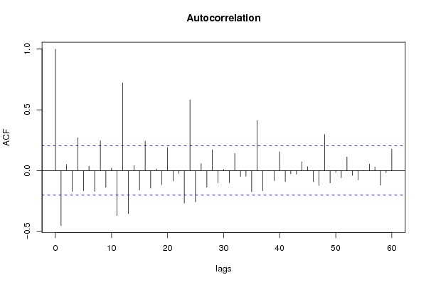
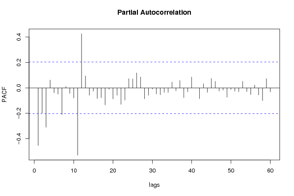
Title produced by software

(Partial) Autocorrelation Function

Date of computation

Mon, 22 Dec 2008 09:40:27 -0700

Cite this page as follows

Statistical Computations at FreeStatistics.org, Office for Research Development and Education, URL https://freestatistics.org/blog/index.php?v=date/2008/Dec/22/t1229964059nj06mp41h8r4q50.htm/, Retrieved Thu, 25 Apr 2024 12:40:35 +0000

Statistical Computations at FreeStatistics.org, Office for Research Development and Education, URL https://freestatistics.org/blog/index.php?pk=36136, Retrieved Thu, 25 Apr 2024 12:40:35 +0000

QR Codes:

Paste this QR Code to cite your computation.

Original text written by user:

IsPrivate?

No (this computation is public)

User-defined keywords

Estimated Impact

252

Family? (F = Feedback message, R = changed R code, M = changed R Module, P = changed Parameters, D = changed Data)

-     [Univariate Data Series] [data set] [2008-12-01 19:54:57] [b98453cac15ba1066b407e146608df68]
F   P   [Univariate Data Series] [Herproducering ti...] [2008-12-03 14:38:00] [6fea0e9a9b3b29a63badf2c274e82506]
-   P     [Univariate Data Series] [Identification an...] [2008-12-08 18:55:50] [79c17183721a40a589db5f9f561947d8]
- RMPD      [(Partial) Autocorrelation Function] [ACF Uitvoer] [2008-12-22 16:25:42] [504b73e6de93b01331326637b3288ad4]
-   PD        [(Partial) Autocorrelation Function] [ACF Invoer zonder...] [2008-12-22 16:38:38] [504b73e6de93b01331326637b3288ad4]
-    D            [(Partial) Autocorrelation Function] [ACF Handelsbalans...] [2008-12-22 16:40:27] [ba85d9d0a82357dd3edf208eef933423] [Current]
-   PD              [(Partial) Autocorrelation Function] [ACF Handelsbalans...] [2008-12-22 16:52:55] [504b73e6de93b01331326637b3288ad4] 

Feedback Forum

Post a new message

Dataseries X:

Download CSV

Histogram

Boxplots

Summary of computational transaction
Raw Input	view raw input (R code)
Raw Output	view raw output of R engine
Computing time	1 seconds
R Server	'Gwilym Jenkins' @ 72.249.127.135

\begin{tabular}{lllllllll}
\hline
Summary of computational transaction \tabularnewline
Raw Input & view raw input (R code)  \tabularnewline
Raw Output & view raw output of R engine  \tabularnewline
Computing time & 1 seconds \tabularnewline
R Server & 'Gwilym Jenkins' @ 72.249.127.135 \tabularnewline
\hline
\end{tabular}
%Source: https://freestatistics.org/blog/index.php?pk=36136&T=0

[TABLE]
[ROW][C]Summary of computational transaction[/C][/ROW]
[ROW][C]Raw Input[/C][C]view raw input (R code) [/C][/ROW]
[ROW][C]Raw Output[/C][C]view raw output of R engine [/C][/ROW]
[ROW][C]Computing time[/C][C]1 seconds[/C][/ROW]
[ROW][C]R Server[/C][C]'Gwilym Jenkins' @ 72.249.127.135[/C][/ROW]
[/TABLE]
Source: https://freestatistics.org/blog/index.php?pk=36136&T=0

Globally Unique Identifier (entire table): ba.freestatistics.org/blog/index.php?pk=36136&T=0

As an alternative you can also use a QR Code:

The GUIDs for individual cells are displayed in the table below:

Summary of computational transaction
Raw Input	view raw input (R code)
Raw Output	view raw output of R engine
Computing time	1 seconds
R Server	'Gwilym Jenkins' @ 72.249.127.135

Autocorrelation Function
Time lag k	ACF(k)	T-STAT	P-value
1	-0.453933	-4.3776	1.6e-05
2	0.04881	0.4707	0.319477
3	-0.173288	-1.6711	0.049029
4	0.270322	2.6069	0.005321
5	-0.166943	-1.6099	0.0554
6	0.037081	0.3576	0.36073
7	-0.17243	-1.6629	0.049854
8	0.245752	2.3699	0.009928
9	-0.138505	-1.3357	0.092455
10	0.019821	0.1911	0.424414
11	-0.372118	-3.5886	0.000266
12	0.721387	6.9568	0
13	-0.355692	-3.4302	0.000451
14	0.040965	0.3951	0.346855
15	-0.161043	-1.553	0.061905
16	0.243159	2.3449	0.010579
17	-0.145308	-1.4013	0.082227
18	0.013847	0.1335	0.447029
19	-0.116616	-1.1246	0.131826
20	0.189197	1.8246	0.03564
21	-0.085988	-0.8292	0.204548
22	-0.023248	-0.2242	0.411547
23	-0.268821	-2.5924	0.005534
24	0.582625	5.6186	0
25	-0.258295	-2.4909	0.007258
26	0.056	0.54	0.295229
27	-0.137824	-1.3291	0.093529
28	0.171126	1.6503	0.05113
29	-0.100918	-0.9732	0.166486
30	0.009036	0.0871	0.465374
31	-0.100743	-0.9715	0.166902
32	0.139226	1.3426	0.091327
33	-0.048203	-0.4649	0.321561
34	-0.046198	-0.4455	0.328489
35	-0.17577	-1.6951	0.046705
36	0.412405	3.9771	6.9e-05
37	-0.167426	-1.6146	0.054893
38	-0.001964	-0.0189	0.492463
39	-0.083388	-0.8042	0.211675
40	0.154151	1.4866	0.070255
41	-0.090865	-0.8763	0.191569
42	-0.027259	-0.2629	0.396613
43	-0.030344	-0.2926	0.385231
44	0.072113	0.6954	0.244258
45	0.03125	0.3014	0.381906
46	-0.091861	-0.8859	0.188986
47	-0.123487	-1.1909	0.118369
48	0.297118	2.8653	0.002575
49	-0.10204	-0.984	0.163826
50	-0.015252	-0.1471	0.44169
51	-0.058549	-0.5646	0.286845
52	0.112634	1.0862	0.140097
53	-0.040659	-0.3921	0.347942
54	-0.078114	-0.7533	0.226586
55	0.000242	0.0023	0.499073
56	0.053134	0.5124	0.304792
57	0.028607	0.2759	0.391628
58	-0.120853	-1.1655	0.123405
59	-0.016641	-0.1605	0.436427
60	0.176979	1.7067	0.045605

\begin{tabular}{lllllllll}
\hline
Autocorrelation Function \tabularnewline
Time lag k & ACF(k) & T-STAT & P-value \tabularnewline
1 & -0.453933 & -4.3776 & 1.6e-05 \tabularnewline
2 & 0.04881 & 0.4707 & 0.319477 \tabularnewline
3 & -0.173288 & -1.6711 & 0.049029 \tabularnewline
4 & 0.270322 & 2.6069 & 0.005321 \tabularnewline
5 & -0.166943 & -1.6099 & 0.0554 \tabularnewline
6 & 0.037081 & 0.3576 & 0.36073 \tabularnewline
7 & -0.17243 & -1.6629 & 0.049854 \tabularnewline
8 & 0.245752 & 2.3699 & 0.009928 \tabularnewline
9 & -0.138505 & -1.3357 & 0.092455 \tabularnewline
10 & 0.019821 & 0.1911 & 0.424414 \tabularnewline
11 & -0.372118 & -3.5886 & 0.000266 \tabularnewline
12 & 0.721387 & 6.9568 & 0 \tabularnewline
13 & -0.355692 & -3.4302 & 0.000451 \tabularnewline
14 & 0.040965 & 0.3951 & 0.346855 \tabularnewline
15 & -0.161043 & -1.553 & 0.061905 \tabularnewline
16 & 0.243159 & 2.3449 & 0.010579 \tabularnewline
17 & -0.145308 & -1.4013 & 0.082227 \tabularnewline
18 & 0.013847 & 0.1335 & 0.447029 \tabularnewline
19 & -0.116616 & -1.1246 & 0.131826 \tabularnewline
20 & 0.189197 & 1.8246 & 0.03564 \tabularnewline
21 & -0.085988 & -0.8292 & 0.204548 \tabularnewline
22 & -0.023248 & -0.2242 & 0.411547 \tabularnewline
23 & -0.268821 & -2.5924 & 0.005534 \tabularnewline
24 & 0.582625 & 5.6186 & 0 \tabularnewline
25 & -0.258295 & -2.4909 & 0.007258 \tabularnewline
26 & 0.056 & 0.54 & 0.295229 \tabularnewline
27 & -0.137824 & -1.3291 & 0.093529 \tabularnewline
28 & 0.171126 & 1.6503 & 0.05113 \tabularnewline
29 & -0.100918 & -0.9732 & 0.166486 \tabularnewline
30 & 0.009036 & 0.0871 & 0.465374 \tabularnewline
31 & -0.100743 & -0.9715 & 0.166902 \tabularnewline
32 & 0.139226 & 1.3426 & 0.091327 \tabularnewline
33 & -0.048203 & -0.4649 & 0.321561 \tabularnewline
34 & -0.046198 & -0.4455 & 0.328489 \tabularnewline
35 & -0.17577 & -1.6951 & 0.046705 \tabularnewline
36 & 0.412405 & 3.9771 & 6.9e-05 \tabularnewline
37 & -0.167426 & -1.6146 & 0.054893 \tabularnewline
38 & -0.001964 & -0.0189 & 0.492463 \tabularnewline
39 & -0.083388 & -0.8042 & 0.211675 \tabularnewline
40 & 0.154151 & 1.4866 & 0.070255 \tabularnewline
41 & -0.090865 & -0.8763 & 0.191569 \tabularnewline
42 & -0.027259 & -0.2629 & 0.396613 \tabularnewline
43 & -0.030344 & -0.2926 & 0.385231 \tabularnewline
44 & 0.072113 & 0.6954 & 0.244258 \tabularnewline
45 & 0.03125 & 0.3014 & 0.381906 \tabularnewline
46 & -0.091861 & -0.8859 & 0.188986 \tabularnewline
47 & -0.123487 & -1.1909 & 0.118369 \tabularnewline
48 & 0.297118 & 2.8653 & 0.002575 \tabularnewline
49 & -0.10204 & -0.984 & 0.163826 \tabularnewline
50 & -0.015252 & -0.1471 & 0.44169 \tabularnewline
51 & -0.058549 & -0.5646 & 0.286845 \tabularnewline
52 & 0.112634 & 1.0862 & 0.140097 \tabularnewline
53 & -0.040659 & -0.3921 & 0.347942 \tabularnewline
54 & -0.078114 & -0.7533 & 0.226586 \tabularnewline
55 & 0.000242 & 0.0023 & 0.499073 \tabularnewline
56 & 0.053134 & 0.5124 & 0.304792 \tabularnewline
57 & 0.028607 & 0.2759 & 0.391628 \tabularnewline
58 & -0.120853 & -1.1655 & 0.123405 \tabularnewline
59 & -0.016641 & -0.1605 & 0.436427 \tabularnewline
60 & 0.176979 & 1.7067 & 0.045605 \tabularnewline
\hline
\end{tabular}
%Source: https://freestatistics.org/blog/index.php?pk=36136&T=1

[TABLE]
[ROW][C]Autocorrelation Function[/C][/ROW]
[ROW][C]Time lag k[/C][C]ACF(k)[/C][C]T-STAT[/C][C]P-value[/C][/ROW]
[ROW][C]1[/C][C]-0.453933[/C][C]-4.3776[/C][C]1.6e-05[/C][/ROW]
[ROW][C]2[/C][C]0.04881[/C][C]0.4707[/C][C]0.319477[/C][/ROW]
[ROW][C]3[/C][C]-0.173288[/C][C]-1.6711[/C][C]0.049029[/C][/ROW]
[ROW][C]4[/C][C]0.270322[/C][C]2.6069[/C][C]0.005321[/C][/ROW]
[ROW][C]5[/C][C]-0.166943[/C][C]-1.6099[/C][C]0.0554[/C][/ROW]
[ROW][C]6[/C][C]0.037081[/C][C]0.3576[/C][C]0.36073[/C][/ROW]
[ROW][C]7[/C][C]-0.17243[/C][C]-1.6629[/C][C]0.049854[/C][/ROW]
[ROW][C]8[/C][C]0.245752[/C][C]2.3699[/C][C]0.009928[/C][/ROW]
[ROW][C]9[/C][C]-0.138505[/C][C]-1.3357[/C][C]0.092455[/C][/ROW]
[ROW][C]10[/C][C]0.019821[/C][C]0.1911[/C][C]0.424414[/C][/ROW]
[ROW][C]11[/C][C]-0.372118[/C][C]-3.5886[/C][C]0.000266[/C][/ROW]
[ROW][C]12[/C][C]0.721387[/C][C]6.9568[/C][C]0[/C][/ROW]
[ROW][C]13[/C][C]-0.355692[/C][C]-3.4302[/C][C]0.000451[/C][/ROW]
[ROW][C]14[/C][C]0.040965[/C][C]0.3951[/C][C]0.346855[/C][/ROW]
[ROW][C]15[/C][C]-0.161043[/C][C]-1.553[/C][C]0.061905[/C][/ROW]
[ROW][C]16[/C][C]0.243159[/C][C]2.3449[/C][C]0.010579[/C][/ROW]
[ROW][C]17[/C][C]-0.145308[/C][C]-1.4013[/C][C]0.082227[/C][/ROW]
[ROW][C]18[/C][C]0.013847[/C][C]0.1335[/C][C]0.447029[/C][/ROW]
[ROW][C]19[/C][C]-0.116616[/C][C]-1.1246[/C][C]0.131826[/C][/ROW]
[ROW][C]20[/C][C]0.189197[/C][C]1.8246[/C][C]0.03564[/C][/ROW]
[ROW][C]21[/C][C]-0.085988[/C][C]-0.8292[/C][C]0.204548[/C][/ROW]
[ROW][C]22[/C][C]-0.023248[/C][C]-0.2242[/C][C]0.411547[/C][/ROW]
[ROW][C]23[/C][C]-0.268821[/C][C]-2.5924[/C][C]0.005534[/C][/ROW]
[ROW][C]24[/C][C]0.582625[/C][C]5.6186[/C][C]0[/C][/ROW]
[ROW][C]25[/C][C]-0.258295[/C][C]-2.4909[/C][C]0.007258[/C][/ROW]
[ROW][C]26[/C][C]0.056[/C][C]0.54[/C][C]0.295229[/C][/ROW]
[ROW][C]27[/C][C]-0.137824[/C][C]-1.3291[/C][C]0.093529[/C][/ROW]
[ROW][C]28[/C][C]0.171126[/C][C]1.6503[/C][C]0.05113[/C][/ROW]
[ROW][C]29[/C][C]-0.100918[/C][C]-0.9732[/C][C]0.166486[/C][/ROW]
[ROW][C]30[/C][C]0.009036[/C][C]0.0871[/C][C]0.465374[/C][/ROW]
[ROW][C]31[/C][C]-0.100743[/C][C]-0.9715[/C][C]0.166902[/C][/ROW]
[ROW][C]32[/C][C]0.139226[/C][C]1.3426[/C][C]0.091327[/C][/ROW]
[ROW][C]33[/C][C]-0.048203[/C][C]-0.4649[/C][C]0.321561[/C][/ROW]
[ROW][C]34[/C][C]-0.046198[/C][C]-0.4455[/C][C]0.328489[/C][/ROW]
[ROW][C]35[/C][C]-0.17577[/C][C]-1.6951[/C][C]0.046705[/C][/ROW]
[ROW][C]36[/C][C]0.412405[/C][C]3.9771[/C][C]6.9e-05[/C][/ROW]
[ROW][C]37[/C][C]-0.167426[/C][C]-1.6146[/C][C]0.054893[/C][/ROW]
[ROW][C]38[/C][C]-0.001964[/C][C]-0.0189[/C][C]0.492463[/C][/ROW]
[ROW][C]39[/C][C]-0.083388[/C][C]-0.8042[/C][C]0.211675[/C][/ROW]
[ROW][C]40[/C][C]0.154151[/C][C]1.4866[/C][C]0.070255[/C][/ROW]
[ROW][C]41[/C][C]-0.090865[/C][C]-0.8763[/C][C]0.191569[/C][/ROW]
[ROW][C]42[/C][C]-0.027259[/C][C]-0.2629[/C][C]0.396613[/C][/ROW]
[ROW][C]43[/C][C]-0.030344[/C][C]-0.2926[/C][C]0.385231[/C][/ROW]
[ROW][C]44[/C][C]0.072113[/C][C]0.6954[/C][C]0.244258[/C][/ROW]
[ROW][C]45[/C][C]0.03125[/C][C]0.3014[/C][C]0.381906[/C][/ROW]
[ROW][C]46[/C][C]-0.091861[/C][C]-0.8859[/C][C]0.188986[/C][/ROW]
[ROW][C]47[/C][C]-0.123487[/C][C]-1.1909[/C][C]0.118369[/C][/ROW]
[ROW][C]48[/C][C]0.297118[/C][C]2.8653[/C][C]0.002575[/C][/ROW]
[ROW][C]49[/C][C]-0.10204[/C][C]-0.984[/C][C]0.163826[/C][/ROW]
[ROW][C]50[/C][C]-0.015252[/C][C]-0.1471[/C][C]0.44169[/C][/ROW]
[ROW][C]51[/C][C]-0.058549[/C][C]-0.5646[/C][C]0.286845[/C][/ROW]
[ROW][C]52[/C][C]0.112634[/C][C]1.0862[/C][C]0.140097[/C][/ROW]
[ROW][C]53[/C][C]-0.040659[/C][C]-0.3921[/C][C]0.347942[/C][/ROW]
[ROW][C]54[/C][C]-0.078114[/C][C]-0.7533[/C][C]0.226586[/C][/ROW]
[ROW][C]55[/C][C]0.000242[/C][C]0.0023[/C][C]0.499073[/C][/ROW]
[ROW][C]56[/C][C]0.053134[/C][C]0.5124[/C][C]0.304792[/C][/ROW]
[ROW][C]57[/C][C]0.028607[/C][C]0.2759[/C][C]0.391628[/C][/ROW]
[ROW][C]58[/C][C]-0.120853[/C][C]-1.1655[/C][C]0.123405[/C][/ROW]
[ROW][C]59[/C][C]-0.016641[/C][C]-0.1605[/C][C]0.436427[/C][/ROW]
[ROW][C]60[/C][C]0.176979[/C][C]1.7067[/C][C]0.045605[/C][/ROW]
[/TABLE]
Source: https://freestatistics.org/blog/index.php?pk=36136&T=1

Globally Unique Identifier (entire table): ba.freestatistics.org/blog/index.php?pk=36136&T=1

As an alternative you can also use a QR Code:

The GUIDs for individual cells are displayed in the table below:

Autocorrelation Function
Time lag k	ACF(k)	T-STAT	P-value
1	-0.453933	-4.3776	1.6e-05
2	0.04881	0.4707	0.319477
3	-0.173288	-1.6711	0.049029
4	0.270322	2.6069	0.005321
5	-0.166943	-1.6099	0.0554
6	0.037081	0.3576	0.36073
7	-0.17243	-1.6629	0.049854
8	0.245752	2.3699	0.009928
9	-0.138505	-1.3357	0.092455
10	0.019821	0.1911	0.424414
11	-0.372118	-3.5886	0.000266
12	0.721387	6.9568	0
13	-0.355692	-3.4302	0.000451
14	0.040965	0.3951	0.346855
15	-0.161043	-1.553	0.061905
16	0.243159	2.3449	0.010579
17	-0.145308	-1.4013	0.082227
18	0.013847	0.1335	0.447029
19	-0.116616	-1.1246	0.131826
20	0.189197	1.8246	0.03564
21	-0.085988	-0.8292	0.204548
22	-0.023248	-0.2242	0.411547
23	-0.268821	-2.5924	0.005534
24	0.582625	5.6186	0
25	-0.258295	-2.4909	0.007258
26	0.056	0.54	0.295229
27	-0.137824	-1.3291	0.093529
28	0.171126	1.6503	0.05113
29	-0.100918	-0.9732	0.166486
30	0.009036	0.0871	0.465374
31	-0.100743	-0.9715	0.166902
32	0.139226	1.3426	0.091327
33	-0.048203	-0.4649	0.321561
34	-0.046198	-0.4455	0.328489
35	-0.17577	-1.6951	0.046705
36	0.412405	3.9771	6.9e-05
37	-0.167426	-1.6146	0.054893
38	-0.001964	-0.0189	0.492463
39	-0.083388	-0.8042	0.211675
40	0.154151	1.4866	0.070255
41	-0.090865	-0.8763	0.191569
42	-0.027259	-0.2629	0.396613
43	-0.030344	-0.2926	0.385231
44	0.072113	0.6954	0.244258
45	0.03125	0.3014	0.381906
46	-0.091861	-0.8859	0.188986
47	-0.123487	-1.1909	0.118369
48	0.297118	2.8653	0.002575
49	-0.10204	-0.984	0.163826
50	-0.015252	-0.1471	0.44169
51	-0.058549	-0.5646	0.286845
52	0.112634	1.0862	0.140097
53	-0.040659	-0.3921	0.347942
54	-0.078114	-0.7533	0.226586
55	0.000242	0.0023	0.499073
56	0.053134	0.5124	0.304792
57	0.028607	0.2759	0.391628
58	-0.120853	-1.1655	0.123405
59	-0.016641	-0.1605	0.436427
60	0.176979	1.7067	0.045605

Partial Autocorrelation Function
Time lag k	PACF(k)	T-STAT	P-value
1	-0.453933	-4.3776	1.6e-05
2	-0.198056	-1.91	0.029609
3	-0.310234	-2.9918	0.001775
4	0.061665	0.5947	0.276752
5	-0.039051	-0.3766	0.353665
6	-0.049142	-0.4739	0.318339
7	-0.2101	-2.0261	0.022808
8	0.010607	0.1023	0.459373
9	-0.043528	-0.4198	0.337811
10	-0.080085	-0.7723	0.220943
11	-0.529852	-5.1097	1e-06
12	0.425568	4.104	4.4e-05
13	0.093992	0.9064	0.183527
14	-0.058533	-0.5645	0.286896
15	-0.02676	-0.2581	0.398465
16	-0.084125	-0.8113	0.20964
17	-0.078311	-0.7552	0.226019
18	-0.134024	-1.2925	0.099696
19	-0.011097	-0.107	0.457502
20	-0.087028	-0.8393	0.201736
21	-0.057796	-0.5574	0.289307
22	-0.130131	-1.2549	0.106322
23	-0.096565	-0.9312	0.177072
24	0.07291	0.7031	0.241868
25	0.070995	0.6846	0.247635
26	0.11775	1.1355	0.129533
27	0.08596	0.829	0.204622
28	-0.086414	-0.8333	0.203393
29	-0.058662	-0.5657	0.286475
30	-0.00913	-0.088	0.465016
31	-0.048516	-0.4679	0.320486
32	-0.055171	-0.5321	0.297979
33	-0.035388	-0.3413	0.366835
34	-0.03651	-0.3521	0.362785
35	0.045575	0.4395	0.330656
36	-0.023454	-0.2262	0.410779
37	0.057627	0.5557	0.289865
38	-0.077368	-0.7461	0.228742
39	-0.031479	-0.3036	0.381064
40	0.085301	0.8226	0.206416
41	-0.000439	-0.0042	0.498314
42	-0.085508	-0.8246	0.205851
43	0.032306	0.3115	0.37804
44	-0.03517	-0.3392	0.367624
45	0.074357	0.7171	0.237564
46	0.050886	0.4907	0.312388
47	-0.025902	-0.2498	0.40165
48	-0.018188	-0.1754	0.430572
49	-0.073888	-0.7126	0.238954
50	-0.011936	-0.1151	0.454305
51	-0.026737	-0.2578	0.398548
52	-0.031161	-0.3005	0.382231
53	0.05101	0.4919	0.311966
54	-0.02963	-0.2857	0.387855
55	-0.053731	-0.5182	0.302788
56	0.021898	0.2112	0.416607
57	-0.055859	-0.5387	0.295694
58	-0.100118	-0.9655	0.168398
59	0.072138	0.6957	0.244185
60	-0.032645	-0.3148	0.376802

\begin{tabular}{lllllllll}
\hline
Partial Autocorrelation Function \tabularnewline
Time lag k & PACF(k) & T-STAT & P-value \tabularnewline
1 & -0.453933 & -4.3776 & 1.6e-05 \tabularnewline
2 & -0.198056 & -1.91 & 0.029609 \tabularnewline
3 & -0.310234 & -2.9918 & 0.001775 \tabularnewline
4 & 0.061665 & 0.5947 & 0.276752 \tabularnewline
5 & -0.039051 & -0.3766 & 0.353665 \tabularnewline
6 & -0.049142 & -0.4739 & 0.318339 \tabularnewline
7 & -0.2101 & -2.0261 & 0.022808 \tabularnewline
8 & 0.010607 & 0.1023 & 0.459373 \tabularnewline
9 & -0.043528 & -0.4198 & 0.337811 \tabularnewline
10 & -0.080085 & -0.7723 & 0.220943 \tabularnewline
11 & -0.529852 & -5.1097 & 1e-06 \tabularnewline
12 & 0.425568 & 4.104 & 4.4e-05 \tabularnewline
13 & 0.093992 & 0.9064 & 0.183527 \tabularnewline
14 & -0.058533 & -0.5645 & 0.286896 \tabularnewline
15 & -0.02676 & -0.2581 & 0.398465 \tabularnewline
16 & -0.084125 & -0.8113 & 0.20964 \tabularnewline
17 & -0.078311 & -0.7552 & 0.226019 \tabularnewline
18 & -0.134024 & -1.2925 & 0.099696 \tabularnewline
19 & -0.011097 & -0.107 & 0.457502 \tabularnewline
20 & -0.087028 & -0.8393 & 0.201736 \tabularnewline
21 & -0.057796 & -0.5574 & 0.289307 \tabularnewline
22 & -0.130131 & -1.2549 & 0.106322 \tabularnewline
23 & -0.096565 & -0.9312 & 0.177072 \tabularnewline
24 & 0.07291 & 0.7031 & 0.241868 \tabularnewline
25 & 0.070995 & 0.6846 & 0.247635 \tabularnewline
26 & 0.11775 & 1.1355 & 0.129533 \tabularnewline
27 & 0.08596 & 0.829 & 0.204622 \tabularnewline
28 & -0.086414 & -0.8333 & 0.203393 \tabularnewline
29 & -0.058662 & -0.5657 & 0.286475 \tabularnewline
30 & -0.00913 & -0.088 & 0.465016 \tabularnewline
31 & -0.048516 & -0.4679 & 0.320486 \tabularnewline
32 & -0.055171 & -0.5321 & 0.297979 \tabularnewline
33 & -0.035388 & -0.3413 & 0.366835 \tabularnewline
34 & -0.03651 & -0.3521 & 0.362785 \tabularnewline
35 & 0.045575 & 0.4395 & 0.330656 \tabularnewline
36 & -0.023454 & -0.2262 & 0.410779 \tabularnewline
37 & 0.057627 & 0.5557 & 0.289865 \tabularnewline
38 & -0.077368 & -0.7461 & 0.228742 \tabularnewline
39 & -0.031479 & -0.3036 & 0.381064 \tabularnewline
40 & 0.085301 & 0.8226 & 0.206416 \tabularnewline
41 & -0.000439 & -0.0042 & 0.498314 \tabularnewline
42 & -0.085508 & -0.8246 & 0.205851 \tabularnewline
43 & 0.032306 & 0.3115 & 0.37804 \tabularnewline
44 & -0.03517 & -0.3392 & 0.367624 \tabularnewline
45 & 0.074357 & 0.7171 & 0.237564 \tabularnewline
46 & 0.050886 & 0.4907 & 0.312388 \tabularnewline
47 & -0.025902 & -0.2498 & 0.40165 \tabularnewline
48 & -0.018188 & -0.1754 & 0.430572 \tabularnewline
49 & -0.073888 & -0.7126 & 0.238954 \tabularnewline
50 & -0.011936 & -0.1151 & 0.454305 \tabularnewline
51 & -0.026737 & -0.2578 & 0.398548 \tabularnewline
52 & -0.031161 & -0.3005 & 0.382231 \tabularnewline
53 & 0.05101 & 0.4919 & 0.311966 \tabularnewline
54 & -0.02963 & -0.2857 & 0.387855 \tabularnewline
55 & -0.053731 & -0.5182 & 0.302788 \tabularnewline
56 & 0.021898 & 0.2112 & 0.416607 \tabularnewline
57 & -0.055859 & -0.5387 & 0.295694 \tabularnewline
58 & -0.100118 & -0.9655 & 0.168398 \tabularnewline
59 & 0.072138 & 0.6957 & 0.244185 \tabularnewline
60 & -0.032645 & -0.3148 & 0.376802 \tabularnewline
\hline
\end{tabular}
%Source: https://freestatistics.org/blog/index.php?pk=36136&T=2

[TABLE]
[ROW][C]Partial Autocorrelation Function[/C][/ROW]
[ROW][C]Time lag k[/C][C]PACF(k)[/C][C]T-STAT[/C][C]P-value[/C][/ROW]
[ROW][C]1[/C][C]-0.453933[/C][C]-4.3776[/C][C]1.6e-05[/C][/ROW]
[ROW][C]2[/C][C]-0.198056[/C][C]-1.91[/C][C]0.029609[/C][/ROW]
[ROW][C]3[/C][C]-0.310234[/C][C]-2.9918[/C][C]0.001775[/C][/ROW]
[ROW][C]4[/C][C]0.061665[/C][C]0.5947[/C][C]0.276752[/C][/ROW]
[ROW][C]5[/C][C]-0.039051[/C][C]-0.3766[/C][C]0.353665[/C][/ROW]
[ROW][C]6[/C][C]-0.049142[/C][C]-0.4739[/C][C]0.318339[/C][/ROW]
[ROW][C]7[/C][C]-0.2101[/C][C]-2.0261[/C][C]0.022808[/C][/ROW]
[ROW][C]8[/C][C]0.010607[/C][C]0.1023[/C][C]0.459373[/C][/ROW]
[ROW][C]9[/C][C]-0.043528[/C][C]-0.4198[/C][C]0.337811[/C][/ROW]
[ROW][C]10[/C][C]-0.080085[/C][C]-0.7723[/C][C]0.220943[/C][/ROW]
[ROW][C]11[/C][C]-0.529852[/C][C]-5.1097[/C][C]1e-06[/C][/ROW]
[ROW][C]12[/C][C]0.425568[/C][C]4.104[/C][C]4.4e-05[/C][/ROW]
[ROW][C]13[/C][C]0.093992[/C][C]0.9064[/C][C]0.183527[/C][/ROW]
[ROW][C]14[/C][C]-0.058533[/C][C]-0.5645[/C][C]0.286896[/C][/ROW]
[ROW][C]15[/C][C]-0.02676[/C][C]-0.2581[/C][C]0.398465[/C][/ROW]
[ROW][C]16[/C][C]-0.084125[/C][C]-0.8113[/C][C]0.20964[/C][/ROW]
[ROW][C]17[/C][C]-0.078311[/C][C]-0.7552[/C][C]0.226019[/C][/ROW]
[ROW][C]18[/C][C]-0.134024[/C][C]-1.2925[/C][C]0.099696[/C][/ROW]
[ROW][C]19[/C][C]-0.011097[/C][C]-0.107[/C][C]0.457502[/C][/ROW]
[ROW][C]20[/C][C]-0.087028[/C][C]-0.8393[/C][C]0.201736[/C][/ROW]
[ROW][C]21[/C][C]-0.057796[/C][C]-0.5574[/C][C]0.289307[/C][/ROW]
[ROW][C]22[/C][C]-0.130131[/C][C]-1.2549[/C][C]0.106322[/C][/ROW]
[ROW][C]23[/C][C]-0.096565[/C][C]-0.9312[/C][C]0.177072[/C][/ROW]
[ROW][C]24[/C][C]0.07291[/C][C]0.7031[/C][C]0.241868[/C][/ROW]
[ROW][C]25[/C][C]0.070995[/C][C]0.6846[/C][C]0.247635[/C][/ROW]
[ROW][C]26[/C][C]0.11775[/C][C]1.1355[/C][C]0.129533[/C][/ROW]
[ROW][C]27[/C][C]0.08596[/C][C]0.829[/C][C]0.204622[/C][/ROW]
[ROW][C]28[/C][C]-0.086414[/C][C]-0.8333[/C][C]0.203393[/C][/ROW]
[ROW][C]29[/C][C]-0.058662[/C][C]-0.5657[/C][C]0.286475[/C][/ROW]
[ROW][C]30[/C][C]-0.00913[/C][C]-0.088[/C][C]0.465016[/C][/ROW]
[ROW][C]31[/C][C]-0.048516[/C][C]-0.4679[/C][C]0.320486[/C][/ROW]
[ROW][C]32[/C][C]-0.055171[/C][C]-0.5321[/C][C]0.297979[/C][/ROW]
[ROW][C]33[/C][C]-0.035388[/C][C]-0.3413[/C][C]0.366835[/C][/ROW]
[ROW][C]34[/C][C]-0.03651[/C][C]-0.3521[/C][C]0.362785[/C][/ROW]
[ROW][C]35[/C][C]0.045575[/C][C]0.4395[/C][C]0.330656[/C][/ROW]
[ROW][C]36[/C][C]-0.023454[/C][C]-0.2262[/C][C]0.410779[/C][/ROW]
[ROW][C]37[/C][C]0.057627[/C][C]0.5557[/C][C]0.289865[/C][/ROW]
[ROW][C]38[/C][C]-0.077368[/C][C]-0.7461[/C][C]0.228742[/C][/ROW]
[ROW][C]39[/C][C]-0.031479[/C][C]-0.3036[/C][C]0.381064[/C][/ROW]
[ROW][C]40[/C][C]0.085301[/C][C]0.8226[/C][C]0.206416[/C][/ROW]
[ROW][C]41[/C][C]-0.000439[/C][C]-0.0042[/C][C]0.498314[/C][/ROW]
[ROW][C]42[/C][C]-0.085508[/C][C]-0.8246[/C][C]0.205851[/C][/ROW]
[ROW][C]43[/C][C]0.032306[/C][C]0.3115[/C][C]0.37804[/C][/ROW]
[ROW][C]44[/C][C]-0.03517[/C][C]-0.3392[/C][C]0.367624[/C][/ROW]
[ROW][C]45[/C][C]0.074357[/C][C]0.7171[/C][C]0.237564[/C][/ROW]
[ROW][C]46[/C][C]0.050886[/C][C]0.4907[/C][C]0.312388[/C][/ROW]
[ROW][C]47[/C][C]-0.025902[/C][C]-0.2498[/C][C]0.40165[/C][/ROW]
[ROW][C]48[/C][C]-0.018188[/C][C]-0.1754[/C][C]0.430572[/C][/ROW]
[ROW][C]49[/C][C]-0.073888[/C][C]-0.7126[/C][C]0.238954[/C][/ROW]
[ROW][C]50[/C][C]-0.011936[/C][C]-0.1151[/C][C]0.454305[/C][/ROW]
[ROW][C]51[/C][C]-0.026737[/C][C]-0.2578[/C][C]0.398548[/C][/ROW]
[ROW][C]52[/C][C]-0.031161[/C][C]-0.3005[/C][C]0.382231[/C][/ROW]
[ROW][C]53[/C][C]0.05101[/C][C]0.4919[/C][C]0.311966[/C][/ROW]
[ROW][C]54[/C][C]-0.02963[/C][C]-0.2857[/C][C]0.387855[/C][/ROW]
[ROW][C]55[/C][C]-0.053731[/C][C]-0.5182[/C][C]0.302788[/C][/ROW]
[ROW][C]56[/C][C]0.021898[/C][C]0.2112[/C][C]0.416607[/C][/ROW]
[ROW][C]57[/C][C]-0.055859[/C][C]-0.5387[/C][C]0.295694[/C][/ROW]
[ROW][C]58[/C][C]-0.100118[/C][C]-0.9655[/C][C]0.168398[/C][/ROW]
[ROW][C]59[/C][C]0.072138[/C][C]0.6957[/C][C]0.244185[/C][/ROW]
[ROW][C]60[/C][C]-0.032645[/C][C]-0.3148[/C][C]0.376802[/C][/ROW]
[/TABLE]
Source: https://freestatistics.org/blog/index.php?pk=36136&T=2

Globally Unique Identifier (entire table): ba.freestatistics.org/blog/index.php?pk=36136&T=2

As an alternative you can also use a QR Code:

The GUIDs for individual cells are displayed in the table below:

Partial Autocorrelation Function
Time lag k	PACF(k)	T-STAT	P-value
1	-0.453933	-4.3776	1.6e-05
2	-0.198056	-1.91	0.029609
3	-0.310234	-2.9918	0.001775
4	0.061665	0.5947	0.276752
5	-0.039051	-0.3766	0.353665
6	-0.049142	-0.4739	0.318339
7	-0.2101	-2.0261	0.022808
8	0.010607	0.1023	0.459373
9	-0.043528	-0.4198	0.337811
10	-0.080085	-0.7723	0.220943
11	-0.529852	-5.1097	1e-06
12	0.425568	4.104	4.4e-05
13	0.093992	0.9064	0.183527
14	-0.058533	-0.5645	0.286896
15	-0.02676	-0.2581	0.398465
16	-0.084125	-0.8113	0.20964
17	-0.078311	-0.7552	0.226019
18	-0.134024	-1.2925	0.099696
19	-0.011097	-0.107	0.457502
20	-0.087028	-0.8393	0.201736
21	-0.057796	-0.5574	0.289307
22	-0.130131	-1.2549	0.106322
23	-0.096565	-0.9312	0.177072
24	0.07291	0.7031	0.241868
25	0.070995	0.6846	0.247635
26	0.11775	1.1355	0.129533
27	0.08596	0.829	0.204622
28	-0.086414	-0.8333	0.203393
29	-0.058662	-0.5657	0.286475
30	-0.00913	-0.088	0.465016
31	-0.048516	-0.4679	0.320486
32	-0.055171	-0.5321	0.297979
33	-0.035388	-0.3413	0.366835
34	-0.03651	-0.3521	0.362785
35	0.045575	0.4395	0.330656
36	-0.023454	-0.2262	0.410779
37	0.057627	0.5557	0.289865
38	-0.077368	-0.7461	0.228742
39	-0.031479	-0.3036	0.381064
40	0.085301	0.8226	0.206416
41	-0.000439	-0.0042	0.498314
42	-0.085508	-0.8246	0.205851
43	0.032306	0.3115	0.37804
44	-0.03517	-0.3392	0.367624
45	0.074357	0.7171	0.237564
46	0.050886	0.4907	0.312388
47	-0.025902	-0.2498	0.40165
48	-0.018188	-0.1754	0.430572
49	-0.073888	-0.7126	0.238954
50	-0.011936	-0.1151	0.454305
51	-0.026737	-0.2578	0.398548
52	-0.031161	-0.3005	0.382231
53	0.05101	0.4919	0.311966
54	-0.02963	-0.2857	0.387855
55	-0.053731	-0.5182	0.302788
56	0.021898	0.2112	0.416607
57	-0.055859	-0.5387	0.295694
58	-0.100118	-0.9655	0.168398
59	0.072138	0.6957	0.244185
60	-0.032645	-0.3148	0.376802

Figure 1

PNG link

Postscript link

PDF link

Figure 2

PNG link

Postscript link

PDF link

Parameters (Session):

par1 = 60 ; par2 = 1 ; par3 = 1 ; par4 = 0 ; par5 = 12 ;

Parameters (R input):

par1 = 60 ; par2 = 1 ; par3 = 1 ; par4 = 0 ; par5 = 12 ;

R code (references can be found in the software module):

if (par1 == 'Default') {
par1 = 10*log10(length(x))
} else {
par1 <- as.numeric(par1)
}
par2 <- as.numeric(par2)
par3 <- as.numeric(par3)
par4 <- as.numeric(par4)
par5 <- as.numeric(par5)
if (par2 == 0) {
x <- log(x)
} else {
x <- (x ^ par2 - 1) / par2
}
if (par3 > 0) x <- diff(x,lag=1,difference=par3)
if (par4 > 0) x <- diff(x,lag=par5,difference=par4)
bitmap(file='pic1.png')
racf <- acf(x,par1,main='Autocorrelation',xlab='lags',ylab='ACF')
dev.off()
bitmap(file='pic2.png')
rpacf <- pacf(x,par1,main='Partial Autocorrelation',xlab='lags',ylab='PACF')
dev.off()
(myacf <- c(racf$acf))
(mypacf <- c(rpacf$acf))
lengthx <- length(x)
sqrtn <- sqrt(lengthx)
load(file='createtable')
a<-table.start()
a<-table.row.start(a)
a<-table.element(a,'Autocorrelation Function',4,TRUE)
a<-table.row.end(a)
a<-table.row.start(a)
a<-table.element(a,'Time lag k',header=TRUE)
a<-table.element(a,hyperlink('basics.htm','ACF(k)','click here for more information about the Autocorrelation Function'),header=TRUE)
a<-table.element(a,'T-STAT',header=TRUE)
a<-table.element(a,'P-value',header=TRUE)
a<-table.row.end(a)
for (i in 2:(par1+1)) {
a<-table.row.start(a)
a<-table.element(a,i-1,header=TRUE)
a<-table.element(a,round(myacf[i],6))
mytstat <- myacf[i]*sqrtn
a<-table.element(a,round(mytstat,4))
a<-table.element(a,round(1-pt(abs(mytstat),lengthx),6))
a<-table.row.end(a)
}
a<-table.end(a)
table.save(a,file='mytable.tab')
a<-table.start()
a<-table.row.start(a)
a<-table.element(a,'Partial Autocorrelation Function',4,TRUE)
a<-table.row.end(a)
a<-table.row.start(a)
a<-table.element(a,'Time lag k',header=TRUE)
a<-table.element(a,hyperlink('basics.htm','PACF(k)','click here for more information about the Partial Autocorrelation Function'),header=TRUE)
a<-table.element(a,'T-STAT',header=TRUE)
a<-table.element(a,'P-value',header=TRUE)
a<-table.row.end(a)
for (i in 1:par1) {
a<-table.row.start(a)
a<-table.element(a,i,header=TRUE)
a<-table.element(a,round(mypacf[i],6))
mytstat <- mypacf[i]*sqrtn
a<-table.element(a,round(mytstat,4))
a<-table.element(a,round(1-pt(abs(mytstat),lengthx),6))
a<-table.row.end(a)
}
a<-table.end(a)
table.save(a,file='mytable1.tab')

Free Statistics

Description of Statistical Computation

Tree of Dependent Computations

Dataset

Tables (Output of Computation)

Figures (Output of Computation)

Input Parameters & R Code